Basic Elements of Elementary Statistics: Visualizing Data Distributions

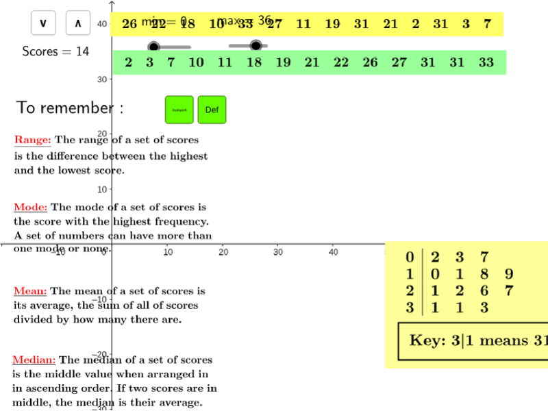
① This GeoGebra example demonstrates how to generate random datasets dynamically and simultaneously display descriptive statistics (mean, median, mode, quartiles, etc.) along with box plots, stem plots, and dot plots to visualize data distributions. ② Core mathematical concepts include measures of central tendency (mean, median, mode), dispersion (range, standard deviation), positional measures (quartiles), and data visualization methods (box plot, stem plot, dot plot). ③ Construction highlights: The Sequence command generates random number sequences, Sort orders them, statistical commands like Mean, Mode, Median, Q1, Q3, Min, Max compute summary values, and BoxPlot, StemPlot, DotPlot create charts; TableText organizes data into tables. Key objects include Random1, Random2, n, max, min, and various cell references. ④ Suitable for high school or introductory college statistics courses, this example helps students understand data distributions, the meaning of statistical measures, and how different charts represent data features. It also serves as an effective classroom demonstration tool for teachers.