
Average vs Instantaneous Rate of Change
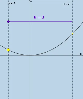
Loading the math board and drawing, please wait…
This example dynamically illustrates the concepts of average and instantaneous rates of change. It involves core math concepts such as derivatives and function graphs. Using GeoGebra commands like Line, Point, Slope, etc., users can explore the rate of change of a function at different points. Suitable for high school and above students and teachers.
GeoGebra Commands & Parameters
Line(A, B) → nPoint(n) → FPoint(g) → ETextfield(a) → InputBox1Textfield(h) → InputBox2Line(A, B) → iSlope(Line[F, B]) → mSlope(Line[E, A]) → m_1Textfield(w) → InputBox3Textfield(f) → InputBox4Point(j) → CIntersect(k, l) → DVector(C, D) → uDistance(C, D) → distanceCD
AI Drawing Prompt Reference
Draw a function graph and mark two points on it, connecting them to form a line segment. Mark the midpoint of the line segment and draw a tangent line from this midpoint to the function graph, marking the intersection point of the tangent line with the graph. Also, draw the secant line connecting the two points on the graph and display its slope. Finally, show the values of the secant slope and tangent slope, as well as the distance between the two points.
The prompt above was compiled from the original drawing commands and is for reference only.