Approximating a Binomial Distribution by a Normal Distribution

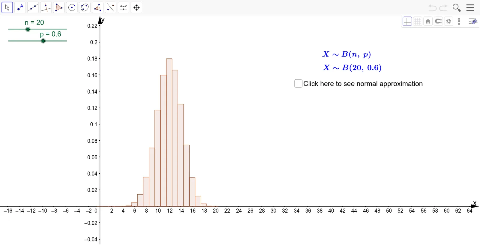
① This example dynamically demonstrates how the binomial probability mass function is approximated by a normal distribution curve as the number of trials n increases, illustrating the central limit theorem visually. ② Core mathematical concepts include binomial distribution, normal distribution, probability density function, mean and standard deviation, and the limiting behavior of distributions. ③ Construction highlights: uses GeoGebra commands BinomialDist to generate the binomial point sequence and Normal to plot the normal curve, with sliders for n and p; objects include n, p, a, f, np, b, c, text6, text7, text2, text3, text8, and d, where np represents the mean and d likely controls the standard deviation or deviation. ④ Suitable for high school to early college probability and statistics courses, serving as a classroom demonstration or self-exploration tool to understand the connection between discrete and continuous distributions.