
Comparing Normal and Binomial Distributions
Loading the math board and drawing, please wait…
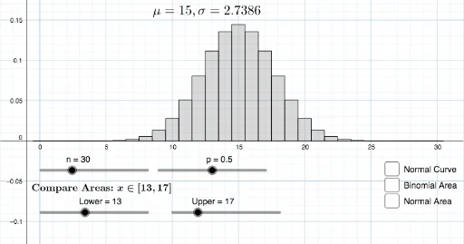
This example demonstrates the comparison of normal and binomial distribution graphs. Key math concepts include probability & statistics, distribution functions, linear regression, and random experiments. It is constructed using GeoGebra commands like Normal, BinomialDist, Max, Sequence, Histogram, and Integral, making it suitable for high school and above learners/researchers in mathematics.
GeoGebra Commands & Parameters
Normal((n * p), sqrt(((n * p) * (1 - p))), x, false) → fBinomialDist(n, p, false) → aMax(f, 0, n) → ASequence(BinomialDist[n, p, k, false], k, v, w, 1) → L_1Histogram(Sequence[k, k, v - 0.5, w + 0.5, 1], L_1) → dIntegral(f, v - 0.5, w + 0.5) → c
AI Drawing Prompt Reference
Create a comparison graph of normal and binomial distributions to illustrate concepts in probability and statistics. Include a normal distribution curve and a binomial distribution curve, both adjustable via sliders. The normal curve is shown within the range from 0 to n, while the binomial curve is represented as a series of bar charts within the same range. Calculate and display the integral of the normal curve over this range as well.
The prompt above was compiled from the original drawing commands and is for reference only.