
Animation 279: Geometric Construction of Parallelograms and Trapezoids
Loading the math board and drawing, please wait…
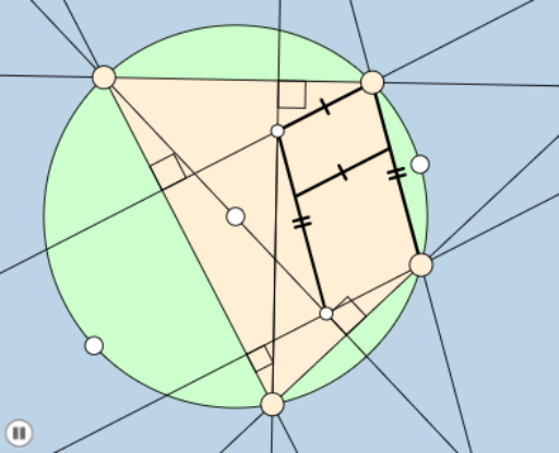
①This GeoGebra example dynamically demonstrates the construction of parallelograms, trapezoids, and triangles, incorporating elements of binomial distribution to blend geometry with probability. ②Core mathematical concepts include properties of parallelograms and trapezoids, triangle construction, circle rotation and arcs, and binomial distribution, along with LCM and GCD relationships. ③Construction highlights: Based on the summary, commands such as Circle, Point, Rotate, CircleArc, Segment, Intersect, Ray, Polygon, Line, OrthogonalLine, Angle, Dilate, Vector, and Translate are used, creating multiple points, lines, circles, polygons, and vectors, with transformations like rotation, translation, and dilation to produce dynamic animations. ④Suitable for middle and high school mathematics, this example serves as a visual aid for geometric constructions, and can also be used to explore connections between geometry and probability, ideal for classroom demonstrations or student self-study of transformations and distributions.
GeoGebra Commands & Parameters
Circle(A_1, B_1) → cPoint(c) → C_1Rotate(C_1, 2°, A_1) → C'CircleArc(A_1, C', C_1) → dPoint(d) → DCircleArc(A_1, D, C_1) → ePoint(e) → CCircleArc(A_1, C, C_1) → fPoint(f) → BCircleArc(A_1, B, C_1) → gPoint(g) → ASegment(D, C) → bSegment(C, B) → hSegment(D, A) → aSegment(A, B) → iCircle(B, (0.2 * Distance[A_1, B_1])) → kCircle(C, (0.2 * Distance[A_1, B_1])) → pCircle(A, (0.2 * Distance[A_1, B_1])) → qCircle(D, (0.2 * Distance[A_1, B_1])) → rIntersect(k, i, 1) → H_1Intersect(k, h, 1) → IIntersect(p, h, 1) → JIntersect(p, b, 1) → KIntersect(r, a, 1) → LIntersect(r, b, 1) → M_1Intersect(q, a, 1) → N_1Intersect(q, i, 1) → OCircle(A_1, B_1) → e_1Ray(D, A) → lPoint(l) → PRay(A, P) → mRay(A, D) → nPoint(n) → QRay(D, Q) → a_1Polygon(A, D, C, B) → poly1, g_2, d_2, e_2, f_2Line(A, D) → sLine(C, B) → tLine(C, D) → f_1Line(B, A) → h_1OrthogonalLine(C, s) → g_1OrthogonalLine(B, m) → i_1OrthogonalLine(D, h_1) → j_1Intersect(g_1, s) → GIntersect(i_1, s) → FOrthogonalLine(A, f_1) → k_1Intersect(f_1, k_1) → EIntersect(h_1, j_1) → HIntersect(i_1, j_1) → NIntersect(k_1, g_1) → MLine(N, M) → l_1Angle(B, F, A) → γAngle(D, G, C) → δAngle(C, E, A) → εAngle(D, H, B) → ζDilate(B, If[0 < o ≤ 1, 1 - o, 0], N) → B'Segment(B, B') → m_1Dilate(C, If[0 < o ≤ 1, 1 - o, 0], M) → C'_1Segment(C, C'_1) → n_1Dilate(D, If[2 < o ≤ 3, 3 - o, 0], N) → D'Dilate(N, If[3 < o ≤ 4, 4 - o, 0], H) → N'Segment(N, N') → p_1Dilate(N, If[1 < o ≤ 2, 2 - o, 0], F) → N'_1Segment(N, N'_1) → q_1Dilate(M, If[1 < o ≤ 2, 2 - o, 0], G) → M'Segment(M, M') → r_1Dilate(A, If[4 < o ≤ 5, 5 - o, 0], M) → A'Segment(A, A') → s_1Dilate(M, If[5 < o ≤ 6, 6 - o, 0], E) → M'_1Segment(M, M'_1) → t_1Dilate(N, If[6 < o ≤ 7, 7 - o, 0], M) → N'_2Segment(N, N'_2) → b_1Segment(N, B) → c_1Line(N, M) → h_2Dilate(N, If[7 < o ≤ 8, 8 - o, 0], B) → N'_3Segment(N, N'_3) → d_1Dilate(N, If[8 < o ≤ 9, 9 - o, 0], B) → N'_4Vector(N, N'_4) → uTranslate(N, u) → N'_5Translate(N'_2, u) → RSegment(N'_5, R) → i_2Dilate(N, If[9 < o ≤ 10, 10 - o, 0], M) → N'_6Vector(N, N'_6) → vTranslate(N, v) → N'_7Translate(N'_3, v) → SSegment(N'_7, S) → j_2Polygon(N, M, C, B) → poly2, n_2, m_2, c_2, b_2Dilate(D, If[2 < o ≤ 3, 3 - o, 0], N) → D'_1Segment(D, D'_1) → j