
Amplitude and Period of Cosine and Sine
Loading the math board and drawing, please wait…
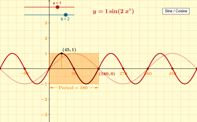
This example demonstrates the graphs of cosine and sine functions, highlighting their amplitude and period variations. Key math concepts include trigonometric functions, amplitude, period, and function graphing. Constructed using GeoGebra commands like Corner, Sequence, Polygon, CurveCartesian, and Vector. Suitable for high school students studying trigonometry and analytical geometry.
GeoGebra Commands & Parameters
Corner(5) → BSequence(Segment[((90 * n), (-dd)), ((90 * n), dd)], n, -2, 6) → list1Sequence(((90 * n), 0), n, -2, 6) → list3Sequence((0, n), n, -3, 3) → list5Sequence(Segment[((-57.3 * dd), n), ((57.3 * dd), n)], n, -3, 3) → list2Sequence(((180 * n / b), 0), n, -9, 9) → list4Sequence(((90 + (180 * n)) / b, 0), n, -9, 9) → list6Polygon((0, (-a)), (360 / b, (-a)), (360 / b, a), (0, a)) → poly1, i, j, k, lCurveCartesian(t, (a * cos((b * t°))), t, Min[0, 360 / b], Max[0, 360 / b]) → dCurveCartesian(t, (a * sin((b * t°))), t, Min[0, 360 / b], Max[0, 360 / b]) → cVector((x(Corner[text21, 1]), (y(Corner[text21, 1]) + y(Corner[text21, 4])) / 2), (Min[0, 360 / b], (y(Corner[text21, 1]) + y(Corner[text21, 4])) / 2)) → uVector((x(Corner[text21, 2]), (y(Corner[text21, 1]) + y(Corner[text21, 4])) / 2), (Max[0, 360 / b], (y(Corner[text21, 1]) + y(Corner[text21, 4])) / 2)) → vVector(((90 / b * ((sc * (-1)) + 1)), 0), ((90 / b * ((sc * (-1)) + 1)), a)) → w
AI Drawing Prompt Reference
Draw the graphs of sine and cosine functions to show their amplitude and period variations. First, draw the coordinate axes and grid lines, then draw the sine and cosine curves. Mark the amplitude and period. Finally, add annotations to explain the amplitude and period.
The prompt above was compiled from the original drawing commands and is for reference only.