Al Horford Parabola: Modeling a Ball with Quadratics

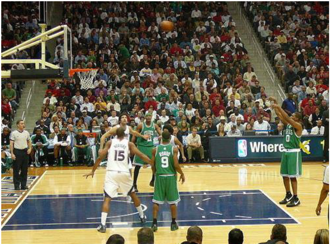
This example demonstrates how a “ball” (or its trajectory/shape behavior) can be modeled using a quadratic curve in GeoGebra. It focuses on the geometric meaning of quadratic functions and how the parabola’s key features—such as special points (e.g., vertex/intersections)—follow from carefully chosen defining elements. The construction also encourages a differential-calculus viewpoint: reasoning about slope and extrema via derivative-based intuition to understand why the curve behaves as it does. In the build, GeoGebra uses constructed objects labeled A, B, C, D, E together with a figure/image object (imagen1) to set up the necessary constraints and then determine the resulting parabola that represents the model. Suitable for upper-secondary to early university use, especially for lessons on graphing, coordinate geometry, curve properties, and introductory modeling with quadratics.