8.2 Orthogonal Diagonalization

Loading the math board and drawing, please wait…

2019-04-15 23:29

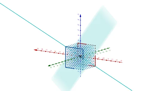
This example demonstrates the orthogonal diagonalization of a matrix, visually representing eigenvectors and eigenvalues through geometric constructs. Core mathematical concepts include orthogonal matrices, eigenvalues, eigenvectors, and diagonalization. GeoGebra commands/objects like ApplyMatrix, Sequence, Point, Polygon, OrthogonalPlane, and Line are used to construct and visualize the matrix transformation and its diagonalization process. Suitable for university-level linear algebra courses to illustrate abstract matrix theory.

GeoGebra Commands & Parameters

ApplyMatrix(M, e_{1}) → t_{1}
ApplyMatrix(M, e_{2}) → t_{2}
ApplyMatrix(M, e_{3}) → t_{3}
Sequence(Sequence[Sequence[(x_{1}, x_{2}, x_{3}), x_{1}, -4, 4, 1], x_{2}, -4, 4, 1], x_{3}, -4, 4, 1) → l1
ApplyMatrix(M, l1) → l1'
Sequence(ApplyMatrix[M, (t, (-2 * t), t)], t, -5, 5, 0.2) → l4
Point(l1') → B
Point(l1') → C
Point(l1') → D
Point(l1') → E
Polygon(B, C, D, E) → q1, b_2, c, d_1, e_4
Point(l1') → F
Point(l1') → G
Point(l1') → H
Point(l1') → J
Polygon(F, G, H, J) → q2, f_1, g_1, h_1, j
ApplyMatrix(M, p1) → p1'
ApplyMatrix(M, p2) → p2'
ApplyMatrix(M, p3) → p3'
OrthogonalPlane((0, 0, 0), Vector[p1 ⊗ p2]) → a
Line((0, 0, 0), p3) → f

AI Drawing Prompt Reference

Visualize the orthogonal diagonalization of a matrix by geometric constructions showing eigenvectors and eigenvalues. Start by plotting the transformed standard basis vectors, then generate a cube in the transformed space and apply the same matrix transformation to observe its deformation. Define an orthogonal plane using three eigenvectors and draw the third one to illustrate the geometric meaning of matrix diagonalization.

The prompt above was compiled from the original drawing commands and is for reference only.