
2D Cone Filling Model
Loading the math board and drawing, please wait…
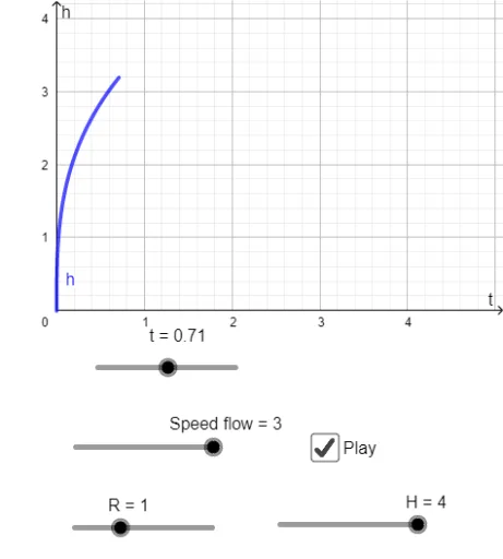
This example demonstrates the filling process of a 2D cone and its geometric properties. It involves core mathematical concepts such as calculus, cone geometry, special points, rhombus, algebra, confidence interval, and median value. The construction utilizes GeoGebra commands and objects like Cone, OrthogonalPlane, IntersectPath, Segment, Circle, OrthogonalLine, Intersect, and Polygon. It is suitable for high school and above, serving as a teaching tool for solid geometry, calculus, and geometric constructions.
GeoGebra Commands & Parameters
Cone(B, (0, 0, 0), R) → cone, c, aOrthogonalPlane(A, zAxis) → planeIntersectPath(plane, cone) → circSegment(Point[circ], A) → rminorCone(A, (0, 0, 0), rminor) → conewater, d, bCircle(B1, R) → c1OrthogonalLine(B1, yAxis) → lperpIntersect(c1, lperp, 1) → C1Intersect(c1, lperp, 2) → C2Segment((0, 0), C1) → s1Segment((0, 0), C2) → s2OrthogonalLine(A1, yAxis) → lperp2Intersect(s1, lperp2) → D1Intersect(s2, lperp2) → D2Polygon((0, 0), D1, C1, C2, D2) → con2d, f, d1, i, c2, d2Polygon((0, 0), D1, D2) → con2dagua, j, k, lSegment(A1, (0, 0)) → heightSegment(B1 + (0, 0.2), C1 + (0, 0.2)) → rrad