
矩形平截头体的体积计算与动态演示
几何画板及绘图内容加载中,请稍等……
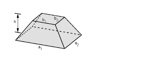
① 本范例通过GeoGebra三维视图动态演示一个矩形平截头体(即被平面截去顶部的四棱锥台)的体积计算过程,直观展示其立体结构与尺寸变化。② 核心数学概念包括立体几何中的棱台体积公式、相似三角形比例关系、导数与极限思想(当顶部截面趋近于底面时退化为棱柱,趋近于顶点时退化为棱锥),以及体积随高度变化的函数关系。③ 作图要点:利用GeoGebra命令如Midpoint(中点)、Translate(平移)、Line(直线)、OrthogonalPlane(正交平面)、Polygon(多边形)、Vector(向量)等构造底面与顶面矩形,通过Segment(线段)连接对应顶点形成棱台,并使用If(条件判断)控制动态参数;对象包括多个顶点(A, B, C, D等)、辅助点(H, I, J等)以及平面和向量,整体支持滑块调节高度与截面位置。④ 适合高中或大学低年级学生用于理解立体几何体积公式的推导,也可作为微积分中“截面法”求体积的直观教具,帮助建立从几何到分析的思维过渡。
GeoGebra 命令及参数
Midpoint(B2', B3) → UTranslate(Prism[H, B2', B2, I], Vector[(0, 0, 0)]) → qMidpoint(B, B1') → VLine(U, V) → pIf(t2 < 0.5, (2 * t2), 1) → t2'If(t2 < 0.5, 0, (2 * (t2 - 0.5))) → t3'Midpoint(B3, B') → KMidpoint(B2, B1') → LLine(L, K) → iSegment(E, B3') → mMidpoint(m) → NOrthogonalPlane(N, m) → n_1Segment(D, B') → kMidpoint(D, B') → MOrthogonalPlane(M, k) → lTranslate(Pyramid[A, D, B', C, B], Vector[(t1 * Vector[B', O])]) → eTranslate(Pyramid[A1, F, B1', E, B1], Vector[(t1 * Vector[B1', O])]) → fTranslate(Pyramid[A3, J, B3', I, B3], Vector[(t1 * Vector[B3', O])]) → gTranslate(Prism[J, B3', B3, C], Vector[(0, 0, 0)]) → jTranslate(Pyramid[A2, G, B2', H, B2], Vector[(t1 * Vector[B2', O])]) → hTranslate(Rotate[Rotate[q, 180°, zAxis], (180° * t2'), p], Vector[(t3' * Vector[B', I])]) → q'Translate(Rotate[Prism[F, B1', B1, G], ((t2' * 180))°, i], Vector[(t3' * Vector[B2', J])]) → oTranslate(Prism[B', B1', B2', B3', B], Vector[(0, 0 - 0)]) → rPolygon(B, B1, B2, B3) → q2, b_1, b1, b2, b3Segment(A, B) → sSegment(A1, B1) → tSegment(A2, B2) → f_1Segment(A3, B3) → g_1Segment(P - (0.5, 0), P - (1.5, 0)) → bPolygon(A, A1, A2, A3) → q1, a, a1, a2, a3Translate(b, Vector[(0, 0, 0), (0, 0, z(B))]) → b'Midpoint(b) → QTranslate(Q, Vector[(0, 0, 0), (0, 0, z(B))]) → Q'Vector(Q, Q') → uVector(Q', Q) → vSegment(H - (0, 1, 0), H - (0, 2, 0)) → cSegment(I - (0, 1, 0), I - (0, 2, 0)) → dVector(Midpoint[c], Midpoint[d]) → wVector(Midpoint[d], Midpoint[c]) → u_1Segment(R - (0, 1, 0), R - (0, 2, 0)) → h_1Segment(S - (0, 1, 0), S - (0, 2, 0)) → i_1Vector(Midpoint[h_1], Midpoint[i_1]) → v_1Vector(Midpoint[i_1], Midpoint[h_1]) → w_1Translate(Polygon[A, B, B3, A3], Vector[(0, 0)]) → q3Translate(Polygon[A, A1, B1, B], Vector[(0, 0)]) → q4Translate(Polygon[A1, A2, B2, B1], Vector[(0, 0)]) → q5Translate(Polygon[A2, A3, B3, B2], Vector[(0, 0)]) → q6If(t0 ≠ 0 ∧ t0 ≠ 1 ∨ t1 ≠ 0 ∧ t1 ≠ 1 ∨ t2 ≠ 0 ∧ t2 ≠ 1, false, true) → showSegment(S + (0.5, 0), S + (1.5, 0)) → j_1Segment(S + (0.5, 0), S + (1.5, 0)) → k_1Segment(T + (0.5, 0), T + (1.5, 0)) → l_1Vector(Midpoint[k_1], Midpoint[l_1]) → a_1Vector(Midpoint[l_1], Midpoint[k_1]) → c_1Segment(C + (0.3, 0), C + (1.2, 0)) → p_1Segment(J + (0.3, 0), J + (1.2, 0)) → m_1Vector(Midpoint[m_1], Midpoint[p_1]) → d_1Vector(Midpoint[p_1], Midpoint[m_1]) → e_1Segment(A3 + (0.3, 0), A3 + (1.2, 0)) → q_1Segment(Midpoint[m_1], Midpoint[q_1]) → r_1Midpoint(r_1) → WSegment(W, Z) → s_1Segment(A3 - (0, 1, 0), A3 - (0, 2, 0)) → t_1Segment(Midpoint[d], Midpoint[t_1]) → v_2Midpoint(v_2) → A_1Segment(B_1, A_1) → f_2