
根据导数信息绘制函数草图
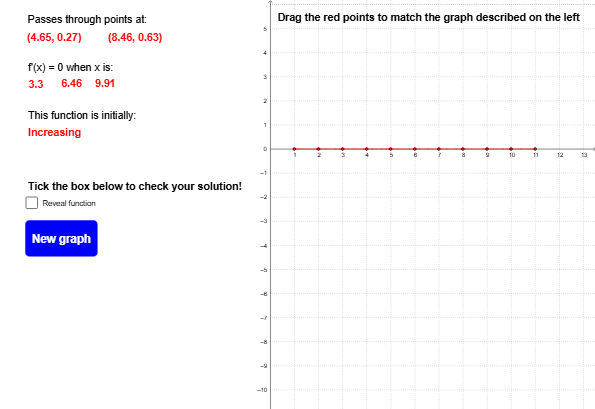
几何画板及绘图内容加载中,请稍等……
本范例演示如何利用函数的导数信息(如极值点、拐点)来手绘或构造函数的大致图像。核心数学概念包括导数、极值、拐点以及函数图像的单调性与凹凸性。作图要点:通过GeoGebra命令如FitPoly拟合多项式,Extremum和TurningPoint自动标记极值点与拐点,并使用Text、If、Segment、Point等命令辅助标注和连线;对象包括多个点(A、B、C等)、分段线段(segA至segK)以及由相邻点构造的抛物线(parABC等),最终形成基于导数信息的草图。适合高中或大学初学微积分的学生,用于理解导数与函数图像特征之间的对应关系。
GeoGebra 命令及参数
Text("This function is initially:") → text8Text("f'(x) = 0 when x is:") → text4If(f'(1) < 0, "Decreasing", "Increasing") → text9Segment((1, -5), (1, 5)) → segASegment((2, -5), (2, 5)) → segBSegment((3, -5), (3, 5)) → segCSegment((4, -5), (4, 5)) → segDSegment((5, -5), (5, 5)) → segESegment((6, -5), (6, 5)) → segFSegment((7, -5), (7, 5)) → segGSegment((8, -5), (8, 5)) → segHSegment((9, -5), (9, 5)) → segISegment((10, -5), (10, 5)) → segJSegment((11, -5), (11, 5)) → segKPoint(segA) → ZAPoint(segB) → ZBPoint(segC) → ZCPoint(segD) → ZDPoint(segE) → ZEPoint(segF) → ZFPoint(segG) → ZGPoint(segH) → ZHPoint(segI) → ZIPoint(segJ) → ZJPoint(segK) → ZKFitPoly({ZA, ZB, ZC}, 2) → parABCFitPoly({ZB, ZC, ZD}, 2) → parBCDFitPoly({ZC, ZD, ZE}, 2) → parCDEFitPoly({ZD, ZE, ZF}, 2) → parDEFFitPoly({ZE, ZF, ZG}, 2) → parEFGFitPoly({ZF, ZG, ZH}, 2) → parFGHFitPoly({ZG, ZH, ZI}, 2) → parGHIFitPoly({ZH, ZI, ZJ}, 2) → parHIJFitPoly({ZI, ZJ, ZK}, 2) → parIJKText("Tick the box below to check your solution!") → text11Text("Passes through points at:") → text1Text("Drag the red points to match the graph described on the left") → text10FitPoly({A, B, C, D, E}, 4) → pExtremum(p, 1, 11) → TP_1, TP_2, TP_3Text(x(TP_1)) → stattext1TurningPoint(p) → IP_1, IP_2Text(IP_1) → inftext1Text(IP_2) → inftext2Text(x(TP_2)) → stattext2Text(x(TP_3)) → stattext3