
简单线性回归
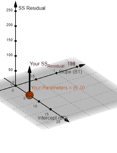
几何画板及绘图内容加载中,请稍等……
①本范例演示了如何使用 GeoGebra 绘制数据点的散点图,并通过最小二乘法拟合出最佳直线;②涉及的核心数学概念包括线性回归、最小二乘法、相关系数、样本均值、协方差等;③作图要点提炼自构造摘要,使用了 Length, mean, Zip, PMCC, SampleSDX, SampleSDY, Point, Line, Slope, Sum, Vector, FitLineY, SumSquaredErrors, RSquare 等命令和对象;④适合高中及以上数学学习者,用于理解数据分析与统计建模的基本原理。
GeoGebra 命令及参数
Length(DataPoints) → SampleSizemean(DataX) → MeanXmean(DataY) → MeanYZip(Vector[(x(A), MeanY), A], A, DataPoints) → FromMeanXZip(Vector[(MeanX, y(A)), A], A, DataPoints) → FromMeanYPMCC(DataPoints) → CorrelationXYSampleSDX(DataPoints) → SXSampleSDY(DataPoints) → SYZip(Point[{A, B}], A, XZ, B, YZ) → DataPointsZZip(Vector[(x(A), 0), A], A, DataPointsZ) → FromMeanXZZip(Vector[(0, y(A)), A], A, DataPointsZ) → FromMeanYZPoint(yAxis) → UserPointALine(UserPointA, UserPointB) → YourLineSlope(YourLine) → UserSlopeZip(Vector[(x(A), YourLine(A)), A], A, DataPoints) → UserResidualVectorSum((DataY - UserPredictedY)^(2)) → UserSSResidualVector(UserParameters, (UserIntercept, UserSlope, UserSSResidual)) → uFitLineY(DataPoints) → fSlope(f) → OLSSlopeSumSquaredErrors(DataPoints, f) → OLSSSResidualVector(OLSParameters, (OLSIntercept, OLSSlope, OLSSSResidual)) → vRSquare(DataPoints, f) → OLSRsqRSquare(DataPoints, YourLine) → UserRsq
AI 绘图提示语参考
绘制散点图展示数据点,并拟合最佳直线。计算并标注样本均值、协方差、相关系数等统计量。用不同颜色展示基于用户输入和最小二乘法的拟合直线,并计算和比较两种方法的残差平方和与决定系数,直观体现线性回归原理。
以上提示语为根据原始绘图命令整理而来,仅供参考。