
简单线性回归与R平方的可视化演示
几何画板及绘图内容加载中,请稍等……
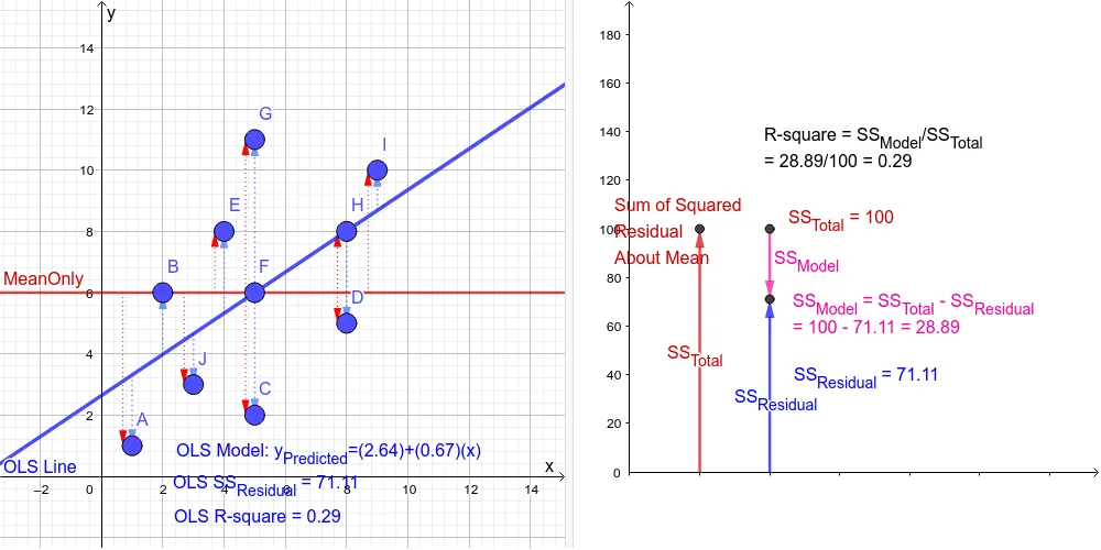
① 本范例通过GeoGebra动态展示简单线性回归中R平方(决定系数)的几何意义,直观呈现数据点与拟合直线之间的关系。② 核心数学概念包括线性回归、最小二乘法、相关系数(PMCC)、协方差、样本标准差以及R平方的计算与解释。③ 作图要点:利用GeoGebra的FitLineY命令生成最佳拟合直线,通过SumSquaredErrors计算残差平方和,使用RSquare得到决定系数;同时构造均值点、数据点、残差向量等对象,并借助滑块或文本显示动态数值变化。④ 适合高中及大学统计学、数据分析课程,用于帮助学生理解回归模型的拟合优度,也可作为教师课堂演示或学生自主探究的素材。
GeoGebra 命令及参数
Length(DataPoints) → SampleSizemean(DataX) → MeanXmean(DataY) → MeanYZip(Vector[(x(A), MeanY), A], A, DataPoints) → FromMeanXZip(Vector[(MeanX, y(A)), A], A, DataPoints) → FromMeanYPMCC(DataPoints) → CorrelationXYSampleSDX(DataPoints) → SXSampleSDY(DataPoints) → SYZip(Point[{A, B}], A, XZ, B, YZ) → DataPointsZZip(Vector[(x(A), 0), A], A, DataPointsZ) → FromMeanXZZip(Vector[(0, y(A)), A], A, DataPointsZ) → FromMeanYZPoint(yAxis) → UserPointALine(UserPointA, UserPointB) → YourLineSlope(YourLine) → UserSlopeSum((DataY - UserPredictedY)^(2)) → UserSSResidualVector(UserParameters, (UserIntercept, UserSlope, UserSSResidual)) → uFitLineY(DataPoints) → fSlope(f) → OLSSlopeSumSquaredErrors(DataPoints, f) → OLSSSResidualVector(OLSParameters, (OLSIntercept, OLSSlope, OLSSSResidual)) → vRSquare(DataPoints, f) → OLSRsqRSquare(DataPoints, YourLine) → UserRsqSumSquaredErrors(DataPoints, MeanOnly) → TotalSSResidualZip(Vector[(x(A), YourLine(A)), A], A, DataPoints) → UserResidualVectorZip(Vector[(x(A), f(A)), A], A, DataPoints) → OLSResidualVectorVector((1, 0), (1, TotalSSResidual)) → VectorTotalSSRVector((2, 0), (2, OLSSSResidual)) → VectorOLSSSRVector((2, TotalSSResidual), (2, OLSSSResidual)) → VectorModelSSRZip(Vector[(x(A) + MDisplace, MeanY), (x(A) + MDisplace, y(A))], A, DataPoints) → MeanResidualVector