
等腰梯形的性质探究
几何画板及绘图内容加载中,请稍等……
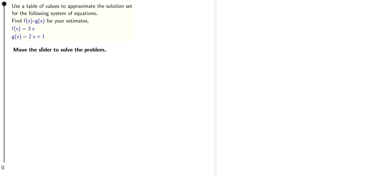
这个范例演示了等腰梯形的性质。涉及的核心数学概念包括线性方程、等腰梯形的性质和逻辑推理。通过使用GeoGebra命令如Corner、Simplify、If等,可以动态展示等腰梯形的构造过程。适合初中及以上学生学习几何作图和逻辑推理。
GeoGebra 命令及参数
LaTeX(steps) → counterLaTeX("\text{Move the slider to solve the problem.}") → text0LaTeX("\text{Use the buttons below to return to the original}\cr\text{problem or randomly generate a similar practice}\cr\text{problem.}") → RandomizationTextCorner(2, 3) → toprightCorner(2, 1) → bottomleftSimplify((ga * x) + gb) → gIf(gb > 0, LaTeX[("+" * gb)], LaTeX[gb]) → gaddIf(ydiff ≟ 0, LaTeX["satisfies"], LaTeX["approximately satisfies"]) → satIf(ydiff ≟ 0, LaTeX["x-coordinate"], LaTeX["approximate x-coordinate"]) → coordIf(ydiff ≟ 0, LaTeX["solution"], LaTeX["approximate solution"]) → solnLaTeX((((("\text{Use a table of values to approximate the solution set}\cr\text{for the following system of equations.}\cr\text{Find }\textcolor{#000099}{f(x) – g(x)}\text{ for your estimates.}\cr\textcolor{#000099}{f(x)=" * f) * "}\cr\textcolor{#000099}{g(x)=") * g) * "}")) → ProblemLaTeX((((("\text{Create a table of values for }\textcolor{#000099}{f(x) = " * f) * "}\text{ and }\cr\textcolor{#000099}{g(x) = ") * g) * "}\text{.}")) → text1Sequence(i, i, (-xscale), xscale) → xvaluesZip(f(j), j, xvalues) → fvaluesZip(g(j), j, xvalues) → gvaluesZip(j - k, j, fvalues, k, gvalues) → fgdiffsTableText({Append[LaTeX["\textcolor{#000099}{x}"], xvalues], Append[LaTeX["\textcolor{#000099}{f(x)}"], fvalues], Append[LaTeX["\textcolor{#000099}{g(x)}"], gvalues], Append[LaTeX["\textcolor{#000099}{f(x)-g(x)}"], fgdiffs]}, "vr") → text2LaTeX("\text{In column }\textcolor{#000099}{f(x) – g(x)}\text{, look for sign changes.}") → text3Sequence(If[sgn(fgdiffs(k)) ≟ sgn(fgdiffs(k + 1)), "F", "T"], k, 1, Length[fgdiffs] - 2) → signChangeLength(signChange \ {"F"}) → numrowsIndexOf("T", signChange) → firstchangeLaTeX((((("\text{There is a sign change from }\textcolor{#000099}{x=" * xvalues(firstchange)) * "}\text{ to }\textcolor{#000099}{x=") * xvalues(firstchange + numrows)) * "}\text{.}")) → text4Sequence(fgdiffs(k), k, firstchange, firstchange + numrows) → fgdiffsSSequence(fvalues(k), k, firstchange, firstchange + numrows) → fvaluesSSequence(gvalues(k), k, firstchange, firstchange + numrows) → gvaluesSSequence(xvalues(k), k, firstchange, firstchange + numrows) → xvaluesSTableText({Append[LaTeX["\textcolor{#000099}{x}"], xvaluesS], Append[LaTeX["\textcolor{#000099}{f(x)}"], fvaluesS], Append[LaTeX["\textcolor{#000099}{g(x)}"], gvaluesS], Append[LaTeX["\textcolor{#000099}{f(x)-g(x)}"], fgdiffsS]}, "vr") → text4bIf(solx ≟ floor(solx), "int", "rat") → versionLaTeX(LaTeX["\text{The sign change occurs between adjacent integers}\cr\text{so look at values in between them.}"]) → text5BSequence(k, k, xvalues(firstchange), xvalues(firstchange) + 1, 0.1) → xvalues2Zip(f(k), k, xvalues2) → fvalues2Zip(g(k), k, xvalues2) → gvalues2Zip(j - k, j, fvalues2, k, gvalues2) → fgdiffs2Sequence(If[sgn(fgdiffs2(k)) ≟ sgn(fgdiffs2(k + 1)), "F", "T"], k, 1, Length[fgdiffs2] - 2) → signChange2LaTeX((((((("\text{Between these points, at }\textcolor{#000099}{x=" * solx) * "}\text{,}\cr\textcolor{#000099}{f(x)-g(x)=") * yapproxf) * "- (") * yapproxg) * ")= 0}\text{.}")) → text5LaTeX((((((((("\text{This tells us the curves }\textcolor{#000099}{f}\text{ and }\textcolor{#000099}{g}\text{ intersect at }\cr\textcolor{#000099}{x = " * xapprox) * "}\text{. The corresponding y-value is}\cr\text{}\textcolor{#000099}{") * yapproxf) * "}\text{. }\text{Therefore, the solution set of this}\cr\text{system is }\textcolor{#000099}{(") * xapprox) * ", ") * yapproxf) * ")}\text{.}")) → text6TableText({Append[LaTeX["\textcolor{#000099}{x}"], xvalues2], Append[LaTeX["\textcolor{#000099}{f(x)}"], fvalues2], Append[LaTeX["\textcolor{#000099}{g(x)}"], gvalues2], Append[LaTeX["\textcolor{#000099}{f(x)-g(x)}"], fgdiffs2]}, "vr") → text5CLaTeX((((((((("\text{This tells us the curves }\textcolor{#000099}{f}\text{ and }\textcolor{#000099}{g}\text{ intersect at }\cr\text{approximately }\textcolor{#000099}{x \approx " * solx) * "}\text{. The corresponding y-value}\cr\text{is approximately }\textcolor{#000099}{") * soly) * "}\text{. }\text{Therefore, the approximate}\cr\text{solution set of this system is }\textcolor{#000099}{(") * solx) * ", ") * soly) * ")}\text{.}")) → text6BLength(signChange2 \ {"F"}) → Sign2CountLaTeX("\text{Since zero once again doesn't show up in the }\cr\textcolor{#000099}{f(x)-g(x)}\text{ values, the actual intersection falls}\cr\text{between table values. The solution above rounds}\cr\text{to the nearest tenth.}") → text6C