
数据分布比较
几何画板及绘图内容加载中,请稍等……
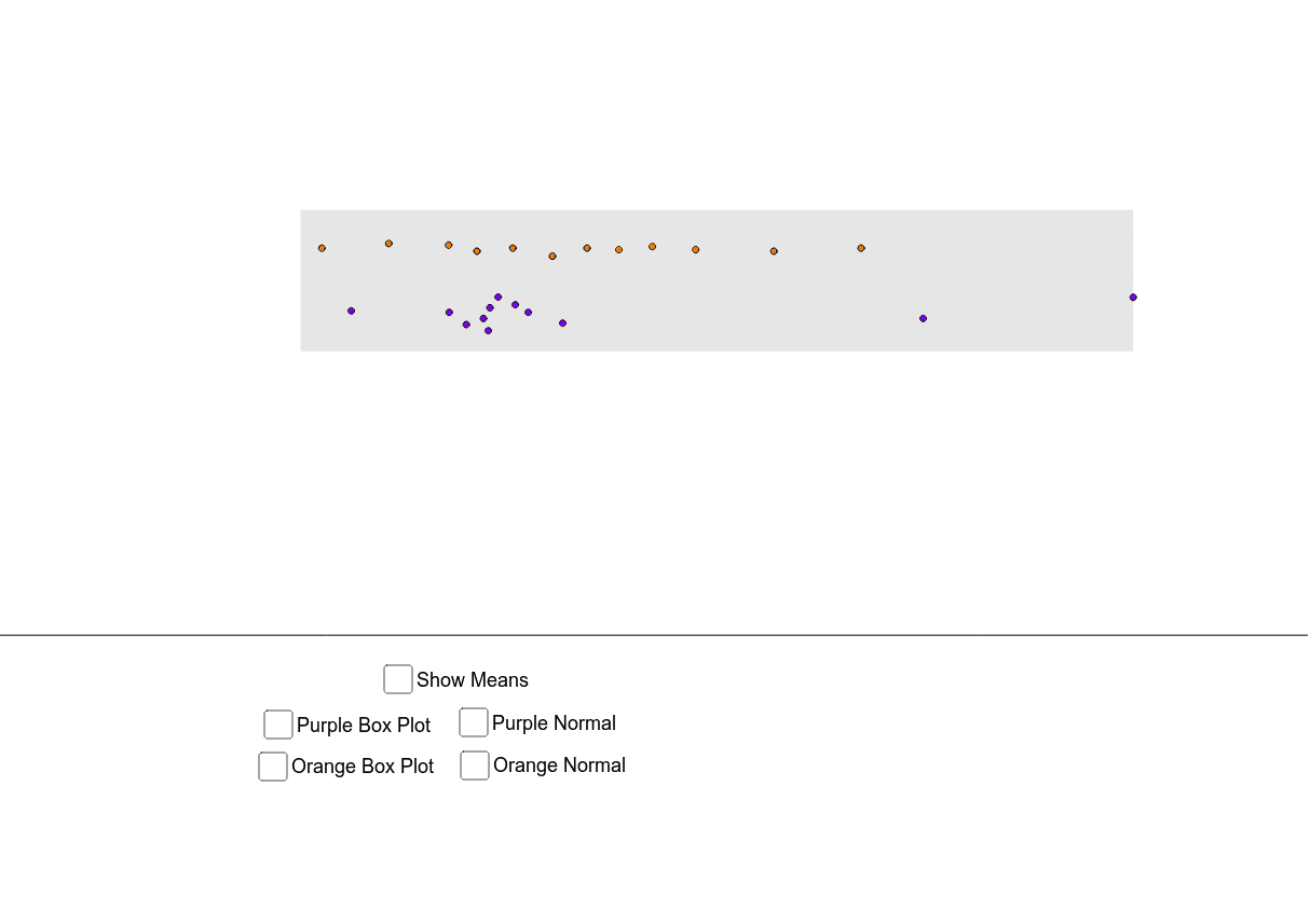
本范例演示如何比较和对比不同数据集的统计中心值(如均值、中位数)和数据可视化(如箱线图、散点图)。通过动态演示,直观展示正态分布、标准差等概念。作图要点:使用了Polygon、PointIn、BoxPlot、MeanX、SDX、Normal、Intersect、Circle、OrthogonalLine、Segment、Mirror等GeoGebra命令和对象来构建和展示数据分布图形。适合高中及以上数学教学,用于概率统计和数据分析课程。
GeoGebra 命令及参数
Polygon(A, B, C, D) → poly1, a, top, c, midPolygon(E, F, G, H) → poly2, e, bottom, g, hPointIn(poly1) → PPointIn(poly1) → QPointIn(poly1) → RPointIn(poly1) → OPointIn(poly1) → A_1PointIn(poly1) → B_1PointIn(poly1) → IPointIn(poly1) → JPointIn(poly1) → KPointIn(poly1) → LPointIn(poly1) → MPointIn(poly1) → NPointIn(poly2) → SPointIn(poly2) → TPointIn(poly2) → UPointIn(poly2) → VPointIn(poly2) → WPointIn(poly2) → ZPointIn(poly2) → C_1PointIn(poly2) → D_1PointIn(poly2) → E_1PointIn(poly2) → F_1PointIn(poly2) → G_1PointIn(poly2) → H_1BoxPlot(7.5, 0.3, x(list_o), true) → boxorangeBoxPlot(6.5, 0.3, x(list_p), true) → boxpurpleMeanX(list_o) → mean_oMeanX(list_p) → mean_pSDX(list_o) → sd_oSDX(list_p) → sd_pNormal(mean_o, sd_o, x) → fNormal(mean_p, sd_p, x) → pIntersect(d, xAxis) → I_1Intersect(b, xAxis) → J_1Circle(I_1, sd_p) → kCircle(I_1, (2 * sd_p)) → sCircle(I_1, (3 * sd_p)) → tCircle(J_1, sd_o) → c_1Circle(J_1, (2 * sd_o)) → d_1Circle(J_1, (3 * sd_o)) → e_1Intersect(k, xAxis) → K_1, L_1Intersect(s, xAxis) → M_1, N_1Intersect(t, xAxis) → O_1, P_1OrthogonalLine(K_1, xAxis) → iOrthogonalLine(M_1, xAxis) → jOrthogonalLine(O_1, xAxis) → lOrthogonalLine(L_1, xAxis) → mOrthogonalLine(N_1, xAxis) → nOrthogonalLine(P_1, xAxis) → a_1Circle(I_1, 6.5) → f_1Intersect(f_1, d) → Q_1, R_1Intersect(r, d, (-3.774228689632889, 2.1243967656986413)) → S_1Intersect(r, i, (-9.407954274837792, 1.2885117717905816)) → T_1Intersect(r, j, (-15.041679860042695, 0.2875058379927696)) → U_1Intersect(r, l, (-20.6754054452476, 0.023599916315999357)) → V_1Intersect(r, m, (1.8594968955720141, 1.2885117717905816)) → W_1Intersect(r, n, (7.493222480776917, 0.2875058379927696)) → Z_1Intersect(r, a_1, (13.126948065981821, 0.023599916315999357)) → A_2Segment(M_1, U_1) → b_1Segment(N_1, Z_1) → j_1Segment(P_1, A_2) → k_1Segment(I_1, Q_1) → h_1Segment(O_1, V_1) → l_1Circle(J_1, 7.5) → p_1Intersect(p_1, b) → B_2, C_2Segment(J_1, B_2) → m_1OrthogonalLine(D_2, xAxis) → n_1OrthogonalLine(E_2, xAxis) → q_1OrthogonalLine(F_2, xAxis) → r_1Mirror(n_1, m_1) → s_1Mirror(q_1, m_1) → t_1Mirror(r_1, m_1) → a_2Intersect(q, s_1, (-7.75562250181825, 1.8221829408666963)) → G_2Intersect(s_1, xAxis) → H_2Intersect(t_1, xAxis) → I_2Intersect(q, t_1, (-11.739372745974084, 0.4065839714153232)) → J_2Intersect(a_2, xAxis) → K_2Intersect(q, a_2, (-15.72312299012992, 0.03337444473412614)) → L_2Intersect(q, n_1, (0.21187798649342193, 1.8221829408666963)) → M_2Intersect(q, q_1, (4.195628230649257, 0.4065839714153229)) → N_2Intersect(q, r_1, (8.179378474805093, 0.03337444473412608)) → O_2Segment(K_2, L_2) → b_2Segment(I_2, J_2) → c_2Segment(N_2, E_2) → d_2Segment(O_2, F_2) → e_2OrthogonalLine(L_1, top) → i_2Intersect(i_2, top) → P_2OrthogonalLine(K_1, top) → j_2Intersect(top, j_2) → Q_2Segment(K_1, Q_2) → g_1Segment(L_1, P_2) → i_1OrthogonalLine(H_2, top) → k_2OrthogonalLine(D_2, top) → l_2Intersect(k_2, top) → R_2Intersect(l_2, top) → S_2Segment(H_2, R_2) → f_2Segment(D_2, S_2) → g_2