
Wrapping Function Demo
Loading the math board and drawing, please wait…
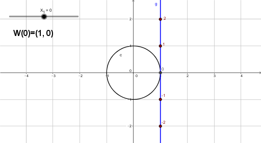
This example demonstrates how the wrapping function maps points on a unit circle to a trajectory in Cartesian coordinates. It involves core mathematical concepts such as the unit circle, parametric curves, trigonometric functions (sine and cosine), and coordinate geometry. The construction uses GeoGebra commands like If and Point, along with variables like X, f, g, h to build parametric equations, and slider animations to show dynamic behavior. Suitable for high school students learning parametric equations, trigonometric graphs, and the properties of wrapping functions, or for introductory calculus instruction.
GeoGebra Commands & Parameters
If(X_1 ≥ 0, Arc[c, (1, 0), (cos(X_1), sin(X_1))], Arc[c, (cos(X_1), sin(X_1)), (1, 0)]) → XIf(X_1 > 0, If[((-1)^(floor(X_1 / π)) * x) < ((-1)^(floor(X_1 / π)) * cos(X_1)), (((-cos(X_1))) / sin(X_1) * (x - cos(X_1))) + sin(X_1)]) → fIf(X_1 ≟ 0, x = 1) → gIf(X_1 > 0, Segment[(1, 0), (1, -10)], X_1 < 0, Segment[(1, 0), (1, 10)]) → hIf(X_1 < 0, If[((-1)^(floor(X_1 / π)) * x) > ((-1)^(floor(X_1 / π)) * cos(X_1)), (((-cos(X_1))) / sin(X_1) * (x - cos(X_1))) + sin(X_1)]) → pIf(0 < X_1 < 1, Point[{cos(X_1) - ((1 - X_1) * sin(X_1)), sin(X_1) + ((1 - X_1) * cos(X_1))}]) → BIf(X_1 ≥ 1, Point[{cos(1), sin(1)}]) → CIf(0 < X_1 < 2, Point[{cos(X_1) - ((2 - X_1) * sin(X_1)), sin(X_1) + ((2 - X_1) * cos(X_1))}]) → DIf(X_1 ≤ 0, Point[{1, 2}]) → EIf(X_1 ≤ 0, Point[{1, 1}]) → AIf(X_1 ≥ 2, Point[{cos(2), sin(2)}]) → FIf(X_1 ≤ 0, Point[{1, 3}]) → GIf(0 < X_1 < 3, Point[{cos(X_1) - ((3 - X_1) * sin(X_1)), sin(X_1) + ((3 - X_1) * cos(X_1))}]) → HIf(X_1 ≥ 3, Point[{cos(3), sin(3)}]) → IIf(X_1 ≥ 0, Point[{1, -1}]) → JIf(-1 < X_1 < 0, Point[{cos(X_1) - ((-1 - X_1) * sin(X_1)), sin(X_1) + ((-1 - X_1) * cos(X_1))}]) → KIf(X_1 ≤ -1, Point[{cos(-1), sin(-1)}]) → LIf(X_1 ≥ 0, Point[{1, -2}]) → MIf(-2 < X_1 < 0, Point[{cos(X_1) - ((-2 - X_1) * sin(X_1)), sin(X_1) + ((-2 - X_1) * cos(X_1))}]) → NIf(X_1 ≤ -2, Point[{cos(-2), sin(-2)}]) → OIf(X_1 ≥ 0, Point[{1, -3}]) → PIf(-3 < X_1 < 0, Point[{cos(X_1) - ((-3 - X_1) * sin(X_1)), sin(X_1) + ((-3 - X_1) * cos(X_1))}]) → QIf(X_1 ≤ -3, Point[{cos(-3), sin(-3)}]) → RIf(X_1 ≥ 0, Point[{1, -4}]) → SIf(-4 < X_1 < 0, Point[{cos(X_1) - ((-4 - X_1) * sin(X_1)), sin(X_1) + ((-4 - X_1) * cos(X_1))}]) → TIf(X_1 ≤ -4, Point[{cos(-4), sin(-4)}]) → UIf(0 < X_1 < 4, Point[{cos(X_1) - ((4 - X_1) * sin(X_1)), sin(X_1) + ((4 - X_1) * cos(X_1))}]) → WIf(X_1 ≥ 4, Point[{cos(4), sin(4)}]) → ZPoint({cos(X_1), sin(X_1)}) → A_1If(X_1 ≤ 0, Point[{1, 4}]) → VIf(X_1 ≤ 0, Point[{1, 5}]) → B_1If(0 < X_1 < 5, Point[{cos(X_1) - ((5 - X_1) * sin(X_1)), sin(X_1) + ((5 - X_1) * cos(X_1))}]) → C_1If(X_1 ≥ 5, Point[{cos(5), sin(5)}]) → D_1If(X_1 ≤ 0, Point[{1, 6}]) → E_1If(0 < X_1 < 6, Point[{cos(X_1) - ((6 - X_1) * sin(X_1)), sin(X_1) + ((6 - X_1) * cos(X_1))}]) → F_1If(X_1 ≥ 6, Point[{cos(6), sin(6)}]) → G_1Point({1, 0}) → H_1