
What is a Function
Loading the math board and drawing, please wait…
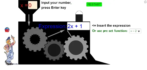
This example dynamically demonstrates the concept of a function, showing the relationship between input and output. Core math concepts include function definition, linear functions, and graph plotting. Construction highlights from the summary involve commands like CurveCartesian, Circle, Polygon, Point, and more. Suitable for middle school students and above for learning functions or classroom demonstrations.
GeoGebra Commands & Parameters
CurveCartesian(x(A) + ((r * (a + (1 / b * tanh((b * sin((n * t) + v)))))) * cos(t + v)), y(A) + ((r * (a + (1 / b * tanh((b * sin((n * t) + v)))))) * sin(t + v)), t, 0, 6.28319) → cCurveCartesian(x(B) + ((R * (a + (1 / b * tanh((b * sin((n * t) - v)))))) * cos(t - v)), y(B) + ((R * (a + (1 / b * tanh((b * sin((n * t) - v)))))) * sin(t - v)), t, 0, 6.28319) → dCircle(B, R + 0.9) → eCircle(A, r + 0.9) → gCircle(A, r + 0.9) → hCurveCartesian(x(A) + ((r * (a + (1 / b * tanh((b * sin((n * t) + v)))))) * cos(t + v)), y(A) + ((r * (a + (1 / b * tanh((b * sin((n * t) + v)))))) * sin(t + v)), t, 0, 6.28319) → iCurveCartesian(x(C) + ((R * (a + (1 / b * tanh((b * sin((n * t) - v)))))) * cos(t - v)), y(C) + ((R * (a + (1 / b * tanh((b * sin((n * t) - v)))))) * sin(t - v)), t, 0, 6.28319) → jCurveCartesian(x(C) + ((r / 2 * (a + (1 / b * tanh((b * sin((n * t) + v)))))) * cos(t + v)), y(C) + ((r / 2 * (a + (1 / b * tanh((b * sin((n * t) + v)))))) * sin(t + v)), t, 0, 6.28319) → oPolygon(D, E, F, G) → poly1, d_1, e_1, f_1, g_1Point(g_1) → HPoint(g_1) → IPolygon(H, I, J, K) → poly2, h_1, i_1, j_1, kPolygon(L, K, J, M) → poly3, l, k_1, j_2, mPoint(f_1) → NPolygon(N, O, P, F) → poly4, n_1, o_1, p, f_2Textfield(s) → ChampTexte1Vector(Q, S) → uTextfield(f) → ChampTexte2Vector(U, V) → wVector(W, Z) → zPolygon(C_1, M, L, D_1) → poly5, c_1, m_1, l_1, d_2Polygon(E_1, F_1, G_1, H_1) → poly6, e_2, f_3, g_2, h_2Semicircle(F_1, G_1) → qMod(v / °, 2) → t_1Semicircle(F_1, G_1) → p_1Segment(A_1, B_1) → a_1LaTeX(f) → textFromFunctionTextToUnicode(textFromFunction) → L_3Text("(" + s + ")") → textFormulaValueTextToUnicode(textFormulaValue) → L_nRemove(Insert[L_n, L_3, IndexOf[120, L_3]], {120}) → L_4Remove(Insert[L_n, L_4, IndexOf[120, L_4]], {120}) → L_5Remove(Insert[L_n, L_5, IndexOf[120, L_5]], {120}) → L_6Remove(Insert[L_n, L_6, IndexOf[120, L_6]], {120}) → L_7Remove(Insert[L_n, L_7, IndexOf[120, L_7]], {120}) → L_8Remove(Insert[L_n, L_8, IndexOf[120, L_8]], {120}) → L_9RemoveUndefined({L_3, L_4, L_5, L_6, L_7, L_8, L_9}) → L_{10}Element(L_{10}, Length[L_{10}]) → L_{11}LaTeX("= " + (UnicodeToText[L_{11}]), true) → textEnumFunction
AI Drawing Prompt Reference
Draw a dynamic function graph to show the relationship between input and output. Start by drawing two circles, then plot two parameterized curves. Next, draw two semicircles and several polygons. Finally, add some points and text to display the function definition.
The prompt above was compiled from the original drawing commands and is for reference only.