
Water Cycle Dynamic Diagram: Merging Trigonometry and Geometric Construction
Loading the math board and drawing, please wait…
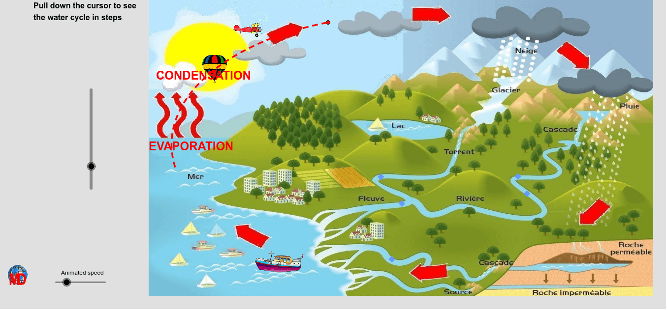
This GeoGebra example presents a visual dynamic diagram of the water cycle, creatively integrating natural phenomena with mathematical graphics. It demonstrates how trigonometric functions, sequences, ellipses, circles, and curve-drawing commands can simulate the cyclic paths of evaporation, condensation, and precipitation. Core mathematical concepts include trigonometric functions (for generating wave-like or cyclic motion), sequences (for creating repeated objects), geometric properties of ellipses and circles (representing water droplets or orbits), and parametric curves (CurveCartesian) to depict flow trajectories. The construction uses commands such as CircumcircleArc to create arcs, Sequence to generate series of points or objects, PolyLine to connect paths, Ellipse to draw elliptical shapes, Point and Intersect to determine key locations, Center to locate circle centers, and CurveCartesian to define custom curves. This example is suitable for middle school to university students, serving as a cross-disciplinary learning tool that links mathematics with earth science. It can also be used as a vivid case for mathematical modeling or dynamic geometry instruction, helping learners understand the application of function graphs and geometric transformations in real-world contexts.
GeoGebra Commands & Parameters
CircumcircleArc(Z_1, A_2, B_2) → gSequence(Sequence[G - ((-0.25 * i), (0.25 * j)), i, 0, Random[3, 6]], j, 0, Random[5, aa]) → liste1Sequence(Sequence[H - ((-0.25 * i), (0.5 * j)), i, 0, Random[3, 6]], j, 0, Random[5, (1.5 * aa)]) → liste2PolyLine(E, I, R, S, T, U, J, K, L, M, N, O, P, Q) → cPolyLine(V, W, U, Z, A_1, B_1, C_1, D_1, E_1, S, T) → dEllipse(D, F_1, F) → ePoint(d) → G_1Point(c) → H_1PolyLine(I_1, J_1, K_1, L_1, M_1, N_1, O_1, P_1) → fPoint(d) → Q_1Point(c) → R_1Point(f) → S_1Point(g) → W_1Sequence(Vector[T_1 + ((0.25 * i), 0), T_1 + ((0.25 * i), ((-cc)) / 8)], i, 0, 5) → liste3Intersect(e, xAxis, 1) → D_2Center(g) → F_2Center(e) → E_2CurveCartesian(x(E_2) + (9.4 * cos((-i))), y(E_2) + (5.25 * sin((-i))), i, -3.32, t) → i
AI Drawing Prompt Reference
Create a dynamic water cycle diagram merging natural phenomena with mathematical graphics. Include an ellipse representing a cyclic orbit, a polyline path connecting multiple points to show rising and falling water vapor, and another polyline for surface runoff. Use an arc to depict cloud formation or evaporation, and a series of regularly spaced points or vectors to simulate falling raindrops. The composition should convey the cyclic process of evaporation, condensation, and precipitation, with curves and geometric shapes interlinked to create a sense of dynamic flow.
The prompt above was compiled from the original drawing commands and is for reference only.