
Volume of Solids by Revolution
Loading the math board and drawing, please wait…
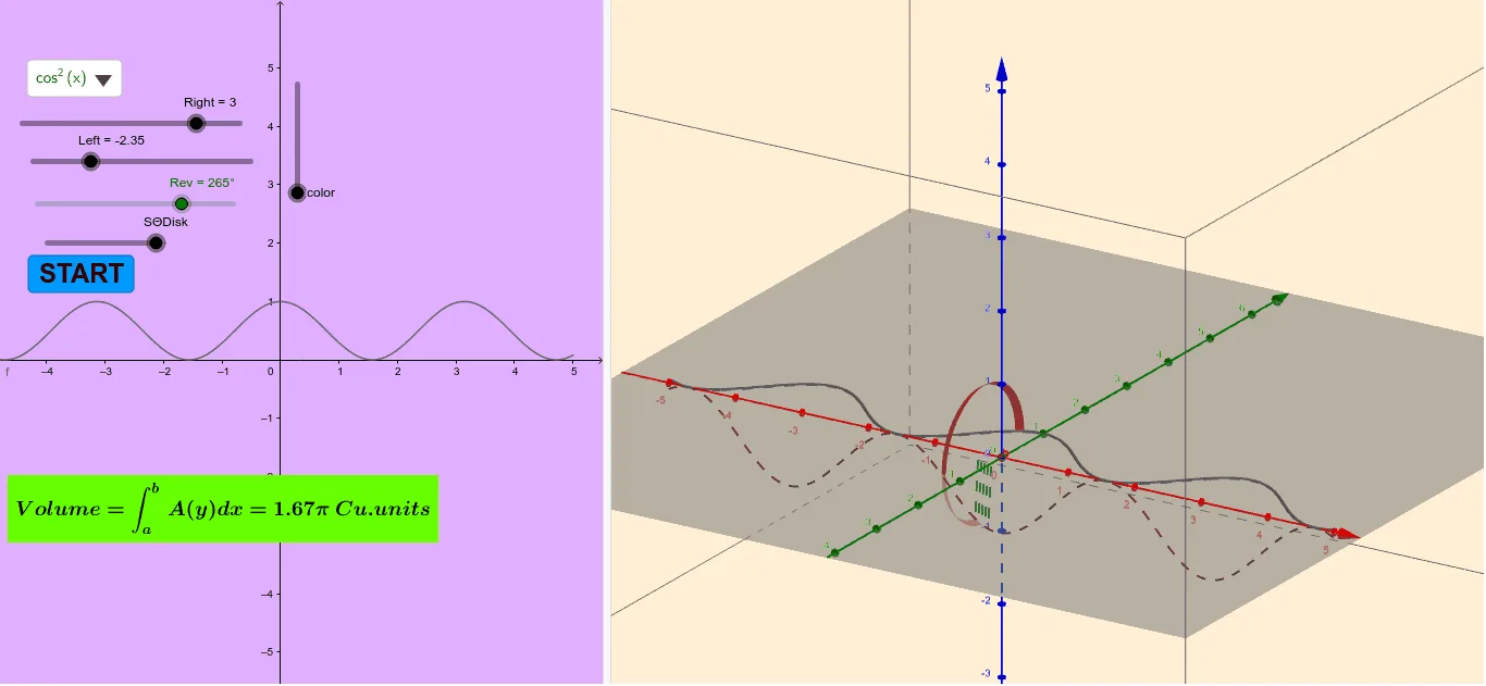
This example demonstrates the calculation of the volume of solids of revolution. Key mathematical concepts include integration and the volume formula for solids of revolution. Using GeoGebra commands such as CurveCartesian, Surface, Sequence, and Integral, the construction of the volume of solids is illustrated. Suitable for high school mathematics education and learning.
GeoGebra Commands & Parameters
CurveCartesian(a, (f(a) * cos(Rev)), (f(a) * sin(Rev)), a, -5, 5) → bSurface(a, (f(a) * cos(β)), (f(a) * sin(β)), a, Left, Right, β, 0, Rev) → cSequence(Segment[(a, 0, 0), (a, (f(a) * cos(Rev)), (f(a) * sin(Rev)))], a, Left, Right, d) → list1Integral(f(x)^(2), Left, Right) → VolumeSurface(a, (f(a) * cos(β)), (f(a) * sin(β)), a, Left + 2, Left + 2.1, β, 0, Rev) → eSequence(Segment[(a, 0, 0), (a, (f(a) * cos(Rev)), (f(a) * sin(Rev)))], a, Left + 2, Left + 2.2, d) → list2Surface(a, (f(a) * cos(β)), (f(a) * sin(β)), a, Left, Right, β, 0, Rev) → gSurface(a, (f(a) * cos(β)), (f(a) * sin(β)), a, Left, Right, β, 0, Rev) → h
AI Drawing Prompt Reference
Illustrate the volume calculation of a solid of revolution by revolving a function around the x-axis, showing the function curve, the generated surface, and the integral area, with auxiliary line segments and surfaces at different positions to demonstrate the volume calculation process.
The prompt above was compiled from the original drawing commands and is for reference only.