
Interactive box plot
Loading the math board and drawing, please wait…
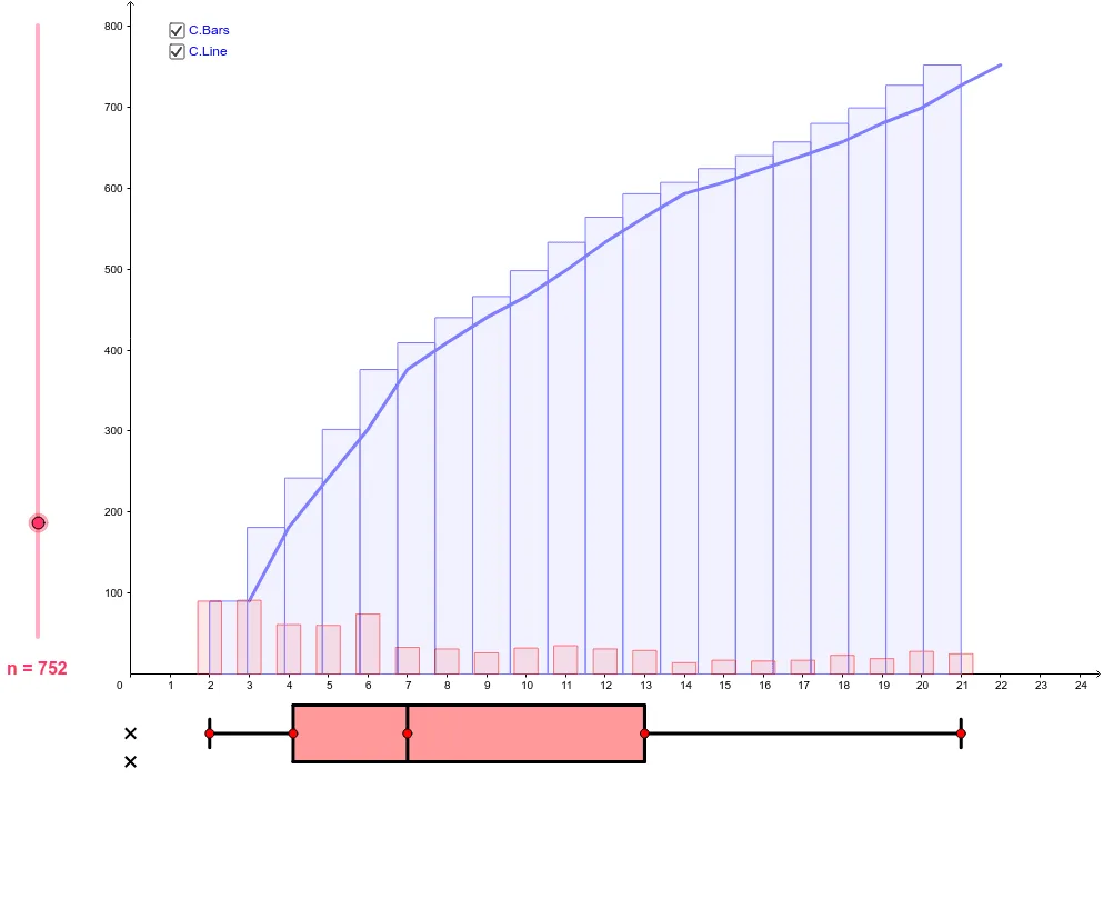
This example demonstrates a dynamic box plot where the box size changes in response to an associated frequency distribution. Key math concepts include frequency distribution, box plot, and data statistics. Construction involves commands/objects like Point, Ray, Segment, Polygon, BarChart, Frequency, Sequence. Suitable for high school mathematics education to visually illustrate data distribution characteristics and statistical changes.
GeoGebra Commands & Parameters
Point(yAxis) → BRay(B, B_1) → sOrthogonalLine(B, s) → g_1Point(g_1) → DRay(D, D_1) → i_1Point(i_1) → ESegment(D, E) → j_1Point(j_1) → FRay(F, F_1) → r_1Point(r_1) → IIf(x(I) < x(E), E, I) → HIf(x(I) < x(E), I, H) → DataUQSegment(F, I) → f_2Point(f_2) → G_1OrthogonalLine(H, yAxis) → pSort(Sequence[floor(RandomUniform[x(DataMin), x(DataLQ)]), k, 1, n]) → IP1RandomSort(Sequence[floor(RandomUniform[x(DataLQ), x(DataMedian)]), k, 1, n]) → IP2RandomSort(Sequence[floor(RandomUniform[x(DataUQ), 1 + x(DataMax)]), k, 1, n]) → IP4RandomSort(Sequence[floor(RandomUniform[x(DataMedian), x(DataUQ)]), k, 1, n]) → IP3RandomJoin({IP1Random, IP2Random, IP3Random, IP4Random}) → DataRandomPointsBarChart(DataRandomPoints, 0.6) → BarChartRandomPointsPoint(s) → CMirror(C, B) → C'_1OrthogonalLine(C, s) → f_1OrthogonalLine(C'_1, s) → h_1Segment(F, E) → k_1OrthogonalLine(I, r_1) → s_1OrthogonalLine(F, r_1) → t_1OrthogonalLine(D, r_1) → a_2OrthogonalLine(E, r_1) → b_2Midpoint(B, C'_1) → JMidpoint(C, B) → RSegment(J, R) → c_2OrthogonalLine(J, a_2) → d_2OrthogonalLine(R, a_2) → e_2Intersect(a_2, d_2) → TIntersect(a_2, e_2) → UIntersect(f_1, t_1) → VIntersect(h_1, t_1) → WIntersect(h_1, s_1) → ZIntersect(f_1, s_1) → A_1Intersect(b_2, e_2) → C_1Intersect(b_2, d_2) → E_1OrthogonalLine(G_1, e_2) → g_2Intersect(h_1, g_2) → H_1Intersect(f_1, g_2) → I_1Segment(T, U) → h_2Segment(D, F) → i_2Segment(W, V) → j_2Segment(V, A_1) → k_2Segment(A_1, Z) → l_2Segment(Z, W) → m_2Segment(H_1, I_1) → n_2Segment(I, E) → p_2Segment(E_1, C_1) → q_2Polygon(W, V, I_1, H_1) → poly3, w, v, i_3, h_3Polygon(I_1, A_1, Z, H_1) → poly4, i_4, a_3, z, h_4Frequency(IP1Random) → Freq1Frequency(IP2Random) → Freq2Frequency(IP3Random) → Freq3Frequency(IP4Random) → Freq4Frequency(DataRandomPoints) → FreqSequence(Sum[Sequence[Element[Freq, i], i, 1, k]], k, 1, Length[Freq]) → FreqCumBarChart(x(DataMin), x(DataMax), FreqCum) → aPolyLine(Sequence[(x(DataMin) + k, Element[FreqCum, k]), k, 1, x(DataMax)]) → b
AI Drawing Prompt Reference
Draw a dynamic box plot where the box size changes based on an associated frequency distribution. Start by plotting a vertical axis and a point, then create rays and perpendicular lines to define the box plot's position. Generate four random points near the minimum, first quartile, median, and third quartile, and use these to construct the box plot. Finally, refine the plot using reflections and intersection calculations to create a complete statistical chart.
The prompt above was compiled from the original drawing commands and is for reference only.