
Frequency and Relative Frequency Distributions
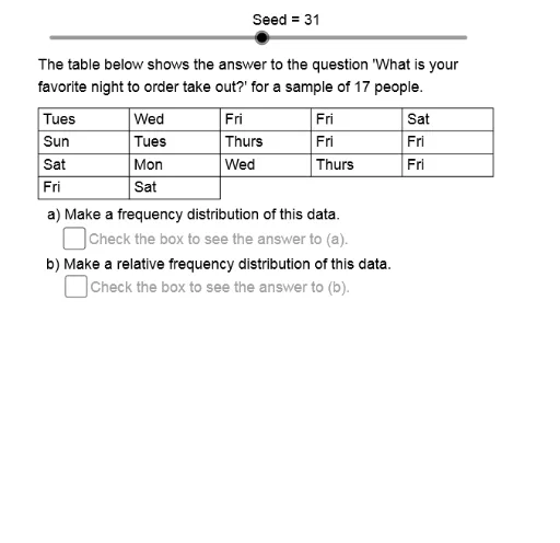
Loading the math board and drawing, please wait…
This example demonstrates how to create frequency and relative frequency histograms using GeoGebra, involving core concepts like data statistics, frequency distribution, and relative frequency calculation. Key GeoGebra commands and objects used include Sequence, Element, Mod, CountIf, Segment, Remove, Text, along with mathematical objects like square roots, cube roots, and various data-related elements. It is suitable for high school students and teachers learning probability and statistics.
GeoGebra Commands & Parameters
Sequence(If[k < 56, If[k < 20, If[k < 8, 1, 2], 3], 4], k, 1, 100) → Sq3Sequence(If[k < 71, If[k < 39, If[k < 26, If[k < 13, 1, 2], 3], 4], 5], k, 1, 100) → Sq2Sequence(If[k < 97, If[k < 90, If[k < 79, If[k < 53, 1, 2], 3], 4], 5], k, 1, 100) → Sq1Sequence(If[k < 80, If[k < 45, If[k < 40, If[k < 25, If[k < 12, If[k < 7, 1, 2], 3], 4], 5], 6], 7], k, 1, 100) → Sq4Element(RtSq, Mod[Seed, 13] + 1) → RateMod(Seed, 7) → StartElement(DataSq, DtNm) → DataMeasSequence(Element[DataMeas, Mod[Start + (Rate * k), 100] + 1], k, 1, Size) → DataACountIf(x ≟ 7, DataA) → Frq7CountIf(x ≟ 6, DataA) → Frq6CountIf(x ≟ 5, DataA) → Frq5CountIf(x ≟ 4, DataA) → Frq4CountIf(x ≟ 3, DataA) → Frq3CountIf(x ≟ 2, DataA) → Frq2CountIf(x ≟ 1, DataA) → Frq1Element(DtCnvSq, DtNm) → DtCnvSequence(Element[DtCnv, Element[DataA, k]], k, 1, Size) → DataBSequence(Text[Element[DataB, k], (1 + ((k - 1) * CW), 13)], k, 1, 5) → DtRw1Sequence(Text[Element[DataB, k], (1 + ((k - 6) * CW), 12.5)], k, 6, 10) → DtRw2Sequence(Text[Element[DataB, k], (1 + ((k - 11) * CW), 12)], k, 11, 15) → DtRw3Segment((0.9, 13.35 - (4 * CH)), (0.9 + (SzNm * CW), 13.35 - (4 * CH))) → BtmLnSequence(Segment[(0.9 + (k * CW), 13.35), (0.9 + (k * CW), If[SzNm ≥ k, 13.35 - (4 * CH), 13.35 - (3 * CH)])], k, 0, 5) → VrtLnsSequence(Text[Element[DataB, k], (1 + ((k - 16) * CW), 11.5)], k, 16, 15 + SzNm) → DtRw4Element(DtLng, DtNm) → CtNmASequence(If[Element[FrqSqA, k] > 0, Element[DtCnv, k], "?"], k, 1, CtNmA) → CtSqARemove(CtSqA, {"?", "?", "?", "?", "?"}) → CtSqBCountIf(x ≠ 0, FrqSqA) → ClsCntRemove(FrqSqA, {0, 0, 0, 0, 0, 0}) → FrqSqBSequence(Element[FrqSqB, k] / Size, k, 1, ClsCnt) → RlFrqSqSequence(Text[Element[CtSqB, k], (1.5, 8.3 - (k * CH))], k, 1, ClsCnt) → ClsTxSequence(Segment[(0.9, 13.35 - (CH * k)), (0.9 + (5 * CW), 13.35 - (CH * k))], k, 0, 3) → HrzLnsSequence(Text[Element[FrqSqB, k], (3.6, 8.3 - (k * CH))], k, 1, ClsCnt) → FrqTxText("Freq.", (3.5, 8.3)) → FrqLbSequence(Text[Element[RlFrqSq, k], (4.7, 8.3 - (k * CH))], k, 1, ClsCnt) → RlFrqTxSequence(Text[Element[FrqSqB, k], (6.1, 8.3 - (k * CH))], k, 1, ClsCnt) → RFClcSqSequence(Text["/", (6.5, 8.3 - (k * CH))], k, 1, ClsCnt) → DvdSqSequence(Text[Size, (6.65, 8.3 - (k * CH))], k, 1, ClsCnt) → SzSq
AI Drawing Prompt Reference
Create a statistical teaching chart with a frequency distribution table and corresponding histogram. Display raw data rows at the top, with numbers arranged in multiple lines. Below, a table lists class intervals, frequencies, relative frequencies (as fractions), and calculation steps. The histogram uses vertical segments to represent frequencies for each class, with a horizontal baseline at the bottom. The layout is clear, suitable for high school probability and statistics instruction.
The prompt above was compiled from the original drawing commands and is for reference only.