
Volume of a Solid of Revolution Around the x-axis by Doug Kuhlmann
Loading the math board and drawing, please wait…
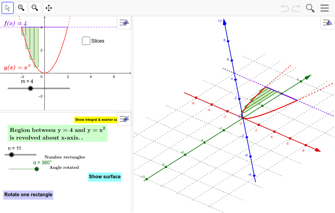
This example provides a dynamic visualization of calculating the volume of a solid generated by rotating a planar region around the x-axis. It focuses on core calculus concepts including the Washer Method and definite integrals. The construction utilizes GeoGebra commands such as Sequence and RectangleSum to approximate the volume via Riemann sums, Rotate and Surface to render the 3D solid, and the Integral command for precise calculation. It is an ideal instructional tool for high school AP Calculus or college-level mathematics students to bridge the gap between 2D integration and 3D spatial volume.
GeoGebra Commands & Parameters
Max({0, m - 1}) → DKPolygon((-2 + (DK * h), g(-2 + ((DK + p) * h))), (-2 + ((DK + 1) * h), g(-2 + ((DK + p) * h))), (-2 + ((DK + 1) * h), f(-2 + ((DK + p) * h))), (-2 + (DK * h), f(-2 + ((DK + p) * h)))) → Rectangle1, j, k, l, m_1RectangleSum(A, -2, -2 + (m * h), m, p) → VolWashSequence(Cylinder[(-2 + (k * h), 0, 0), (-2 + ((k + 1) * h), 0, 0), g(-2 + ((k + p) * h))], k, 0, m - 1) → CISequence(If[Defined[Element[CI, k]], Volume[Element[CI, k]], 0], k, 1, m) → VCISequence(Cylinder[(-2 + (k * h), 0, 0), (-2 + ((k + 1) * h), 0, 0), f(-2 + ((k + p) * h))], k, 0, m - 1) → COSequence(If[Defined[Element[CO, k]], Volume[Element[CO, k]], 0], k, 1, m) → VCORotate(Rectangle1, (-α), c) → RotateRectangle1Surface(u, (g(-2 + ((DK + p) * h)) * cos(β)), (g(-2 + ((DK + p) * h)) * sin(β)), u, -2 + (DK * h), -2 + ((DK + 1) * h), β, 0, α) → Inner1Vector((-2 + ((DK + 1) * h), 0, 0), (-2 + ((DK + 1) * h), g(-2 + ((DK + p) * h)), 0)) → rVector((-2 + (DK * h), 0, 0), (-2 + (DK * h), f(-2 + (DK * h)), 0)) → RRotate(R, (-α), c) → R'Rotate(r, (-α), c) → r'Integral(16 - x^(4), -2, 2) → VolumeIntegralIf(togV ≟ 1, "Hide integral & washer sums", "Show integral & washer sums") → ShowVolIntegralSequence(Polygon[(-2 + (k * h), g(-2 + ((k + p) * h))), (-2 + ((k + 1) * h), g(-2 + ((k + p) * h))), (-2 + ((k + 1) * h), f(-2 + ((k + p) * h))), (-2 + (k * h), f(-2 + ((k + p) * h)))], k, 0, m - 1) → RectanglesRotate(Rectangles, (-α), c) → Rectangles'Surface(u, (f(-2 + ((DK + p) * h)) * cos(β)), (f(-2 + ((DK + p) * h)) * sin(β)), u, -2 + (DK * h), -2 + ((DK + 1) * h), β, 0, α) → Outer1Rotate(f_1, α, xAxis) → f_2Rotate(g_1, α, xAxis) → g_2If(togS ≟ 1, "Hide surface", "Show surface") → ShowSurfaceSurface(u, (f(u) * cos(β)), (f(u) * sin(β)), u, -2, 2, β, 0, 6.283185307179586) → SurfaceOuterSurface(u, (g(u) * cos(β)), (g(u) * sin(β)), u, -2, 2, β, 0, 6.283185307179586) → SurfaceInnerIf(togR ≟ 1, "Rotate one rectangle", "Rotate all rectangles") → RotateOneDiskSequence(Surface[-2 + ((k + u) * h), (4 * cos(β)), (4 * sin(β)), u, 0, 1, β, 0, α], k, 0, m - 1) → OutersSequence(Surface[-2 + ((k + u) * h), (g(-2 + ((k + p) * h)) * cos(β)), (g(-2 + ((k + p) * h)) * sin(β)), u, 0, 1, β, 0, α], k, 0, m - 1) → InnersSequence(Surface[-2 + (k * h), (u * cos(β)), (u * sin(β)), u, g(-2 + ((k + p) * h)), f(-2 + ((k + p) * h)), β, 0, α], k, 0, m - 1) → SidesLeftSequence(Surface[-2 + ((k + 1) * h), (u * cos(β)), (u * sin(β)), u, g(-2 + ((k + p) * h)), f(-2 + ((k + p) * h)), β, 0, α], k, 0, m - 1) → SidesRightSurface(-2 + ((DK + 1) * h), (u * cos(β)), (u * sin(β)), u, g(-2 + ((DK + p) * h)), f(-2 + ((DK + p) * h)), β, 0, α) → Side1RightSurface(-2 + (DK * h), (u * cos(β)), (u * sin(β)), u, g(-2 + ((DK + p) * h)), f(-2 + ((DK + p) * h)), β, 0, α) → Side1Left
AI Drawing Prompt Reference
Create a 3D visualization of a solid of revolution generated by rotating a planar region around the x-axis. The region is bounded between two curves, an outer curve and an inner curve, over the interval [-2,2] on the x-axis. Rotating this region about the x-axis produces a hollow solid with an outer surface from the outer curve and an inner surface from the inner curve. Display multiple rectangular strips representing Riemann sums for approximating the volume using the washer method, each strip rotated to form a thin shell. Highlight one specific rectangle and its rotated 3D counterpart. Also show the exact volume value computed by integration. The scene is instructional, bridging 2D integration and 3D volume.
The prompt above was compiled from the original drawing commands and is for reference only.