
Volume of a Rectangular Frustum
Loading the math board and drawing, please wait…
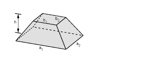
① This GeoGebra example dynamically demonstrates the volume calculation of a rectangular frustum (a truncated rectangular pyramid), showing its 3D structure and how dimensions affect the volume. ② Core mathematical concepts include solid geometry (frustum volume formula), similar triangles for proportional relationships, and the ideas of derivative and limit (as the top face approaches the base, it becomes a prism; as it approaches the apex, it becomes a pyramid). ③ Construction highlights: using GeoGebra commands such as Midpoint, Translate, Line, OrthogonalPlane, Polygon, and Vector to build the base and top rectangles, connecting corresponding vertices with Segment to form the frustum, and using If for conditional dynamic parameters; objects include multiple vertices (A, B, C, D, etc.), auxiliary points (H, I, J, etc.), planes, and vectors, with sliders to adjust height and section position. ④ Suitable for high school or early college students to understand the derivation of volume formulas in solid geometry, and as a visual aid for the 'cross-section method' in calculus, bridging geometric intuition and analytical thinking.
GeoGebra Commands & Parameters
Midpoint(B2', B3) → UTranslate(Prism[H, B2', B2, I], Vector[(0, 0, 0)]) → qMidpoint(B, B1') → VLine(U, V) → pIf(t2 < 0.5, (2 * t2), 1) → t2'If(t2 < 0.5, 0, (2 * (t2 - 0.5))) → t3'Midpoint(B3, B') → KMidpoint(B2, B1') → LLine(L, K) → iSegment(E, B3') → mMidpoint(m) → NOrthogonalPlane(N, m) → n_1Segment(D, B') → kMidpoint(D, B') → MOrthogonalPlane(M, k) → lTranslate(Pyramid[A, D, B', C, B], Vector[(t1 * Vector[B', O])]) → eTranslate(Pyramid[A1, F, B1', E, B1], Vector[(t1 * Vector[B1', O])]) → fTranslate(Pyramid[A3, J, B3', I, B3], Vector[(t1 * Vector[B3', O])]) → gTranslate(Prism[J, B3', B3, C], Vector[(0, 0, 0)]) → jTranslate(Pyramid[A2, G, B2', H, B2], Vector[(t1 * Vector[B2', O])]) → hTranslate(Rotate[Rotate[q, 180°, zAxis], (180° * t2'), p], Vector[(t3' * Vector[B', I])]) → q'Translate(Rotate[Prism[F, B1', B1, G], ((t2' * 180))°, i], Vector[(t3' * Vector[B2', J])]) → oTranslate(Prism[B', B1', B2', B3', B], Vector[(0, 0 - 0)]) → rPolygon(B, B1, B2, B3) → q2, b_1, b1, b2, b3Segment(A, B) → sSegment(A1, B1) → tSegment(A2, B2) → f_1Segment(A3, B3) → g_1Segment(P - (0.5, 0), P - (1.5, 0)) → bPolygon(A, A1, A2, A3) → q1, a, a1, a2, a3Translate(b, Vector[(0, 0, 0), (0, 0, z(B))]) → b'Midpoint(b) → QTranslate(Q, Vector[(0, 0, 0), (0, 0, z(B))]) → Q'Vector(Q, Q') → uVector(Q', Q) → vSegment(H - (0, 1, 0), H - (0, 2, 0)) → cSegment(I - (0, 1, 0), I - (0, 2, 0)) → dVector(Midpoint[c], Midpoint[d]) → wVector(Midpoint[d], Midpoint[c]) → u_1Segment(R - (0, 1, 0), R - (0, 2, 0)) → h_1Segment(S - (0, 1, 0), S - (0, 2, 0)) → i_1Vector(Midpoint[h_1], Midpoint[i_1]) → v_1Vector(Midpoint[i_1], Midpoint[h_1]) → w_1Translate(Polygon[A, B, B3, A3], Vector[(0, 0)]) → q3Translate(Polygon[A, A1, B1, B], Vector[(0, 0)]) → q4Translate(Polygon[A1, A2, B2, B1], Vector[(0, 0)]) → q5Translate(Polygon[A2, A3, B3, B2], Vector[(0, 0)]) → q6If(t0 ≠ 0 ∧ t0 ≠ 1 ∨ t1 ≠ 0 ∧ t1 ≠ 1 ∨ t2 ≠ 0 ∧ t2 ≠ 1, false, true) → showSegment(S + (0.5, 0), S + (1.5, 0)) → j_1Segment(S + (0.5, 0), S + (1.5, 0)) → k_1Segment(T + (0.5, 0), T + (1.5, 0)) → l_1Vector(Midpoint[k_1], Midpoint[l_1]) → a_1Vector(Midpoint[l_1], Midpoint[k_1]) → c_1Segment(C + (0.3, 0), C + (1.2, 0)) → p_1Segment(J + (0.3, 0), J + (1.2, 0)) → m_1Vector(Midpoint[m_1], Midpoint[p_1]) → d_1Vector(Midpoint[p_1], Midpoint[m_1]) → e_1Segment(A3 + (0.3, 0), A3 + (1.2, 0)) → q_1Segment(Midpoint[m_1], Midpoint[q_1]) → r_1Midpoint(r_1) → WSegment(W, Z) → s_1Segment(A3 - (0, 1, 0), A3 - (0, 2, 0)) → t_1Segment(Midpoint[d], Midpoint[t_1]) → v_2Midpoint(v_2) → A_1Segment(B_1, A_1) → f_2