Visualizing the Tangent Plane

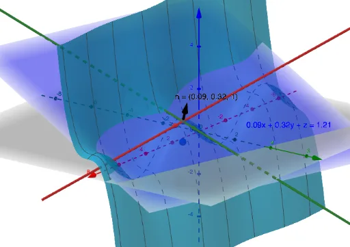
This example demonstrates how to visualize a tangent plane in 3D space. It involves core mathematical concepts such as partial derivatives, tangent planes, and vectors. Key construction points include using GeoGebra commands like PointIn, Derivative, Line, Vector, IntersectPath to construct the tangent plane of function f, and display its normal and tangent vectors. Suitable for university calculus courses or to understand the geometric properties of multivariable functions.