
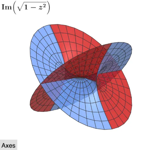
Visualizing the Imaginary Component (1-z^2)^(1/2)
Loading the math board and drawing, please wait…
This example demonstrates the visualization of the imaginary component function (1-z^2)^(1/2) as a 3D surface, exploring its geometric properties and variations. Key math concepts include complex numbers, imaginary parts, function graphs, 3D surfaces, and analytical geometry. GeoGebra commands like Surface, SelectedIndex, ListBranches, and Slider Animation are used to construct the model. Suitable for high school and above students to understand the geometric meaning and visualization of complex function graphs.
GeoGebra Commands & Parameters
SelectedIndex(ListBranches) → indexSurface((u * cos(v)), (u * sin(v)), Im((u * cos(v)), (u * sin(v)), 2, 0), u, 0, 2, v, 0, π - π / 1000) → C0Surface((u * cos(v)), (u * sin(v)), Im((u * cos(v)), (u * sin(v)), 2, 1), u, 0, 2, v, 0, π - π / 1000) → C1Surface((u * cos(v)), (u * sin(v)), Im((u * cos(v)), (u * sin(v)), 2, 0), u, 0, 2, v, (-π), ((-π)) / 1000) → D0Surface((u * cos(v)), (u * sin(v)), Im((u * cos(v)), (u * sin(v)), 2, 1), u, 0, 2, v, (-π), ((-π)) / 1000) → D1
AI Drawing Prompt Reference
Create a 3D surface plot visualizing the imaginary part of the complex function (1-z^2)^(1/2), where z is represented in polar coordinates as u*cos(v) and u*sin(v), with u ranging from 0 to 2 and v from 0 to just below π, showing two distinct branches of the imaginary part and including mirrored branches for v ranging from negative π to just below negative π.
The prompt above was compiled from the original drawing commands and is for reference only.