
Visualizing Subtracting Integers with Vector Geometry
Loading the math board and drawing, please wait…
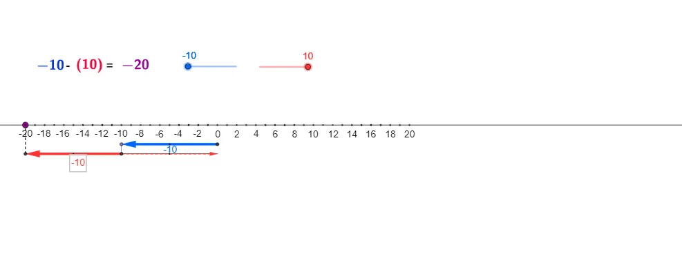
This GeoGebra example demonstrates how subtracting integers can be visualized as operations on directed lengths and 2D vectors. By constructing lines, reference points, and measurable segments, the diagram encodes “integer values” along a chosen direction and shows that the subtraction outcome corresponds to a specific vector difference obtained through geometric transformations. Key math ideas include integers, vectors in 2D (directed magnitude), proportional reasoning via similar triangles, and geometric construction methods that support accurate reading of the result. The construction uses core GeoGebra commands such as Line, Point, Segment, Circle, Intersect, and OrthogonalLine to set up the geometric framework; Vector to represent directed quantities; Translate and Mirror to move and align vectors consistently; and Midpoint to create symmetry/proportion anchors. It is well-suited for middle school to early university learners studying vectors, coordinate/geometry construction, and the connection between arithmetic on integers and geometric/vector interpretation.
GeoGebra Commands & Parameters
Line(A, B) → aPoint(a) → CCircle(C, 4) → kOrthogonalLine(C, a) → dIntersect(k, d, 2) → R_1Intersect(k, d, 1) → J_1Circle(C, 2) → pIntersect(p, d) → I_1, L_5Circle(L_5, 1) → gIntersect(g, d, 1) → N_1Circle(R_1, N_1) → rIntersect(r, d, 2) → S_1OrthogonalLine(N_1, d) → iCircle(M_1, 1) → qIntersect(q, i) → O_1, P_1Vector(I_1, L_1) → vTranslate(O_1, v) → Q_1Mirror(Q_1, O_1) → Z_1Point(a) → DPoint(a) → EPoint(a) → FPoint(a) → GPoint(a) → HPoint(a) → IPoint(a) → JPoint(a) → KPoint(a) → LPoint(a) → MPoint(a) → NPoint(a) → OPoint(a) → PPoint(a) → QPoint(a) → RPoint(a) → SPoint(a) → TPoint(a) → UPoint(a) → VPoint(a) → WPoint(a) → YPoint(a) → ZPoint(a) → A_1Point(a) → B_1Point(a) → C_1Point(a) → D_1Point(a) → E_1Point(a) → F_1Point(a) → G_1Point(a) → H_1OrthogonalLine(I_1, d) → eOrthogonalLine(L_5, d) → hOrthogonalLine(J_1, d) → fVector(J_1, K_1) → uVector(L_5, M_1) → wVector(O_1, Q_1) → zOrthogonalLine(S_1, d) → jVector(S_1, T_1) → lSegment(J_1, S_1) → mSegment(M_1, O_1) → tOrthogonalLine(K_1, a) → nIntersect(n, a) → U_1OrthogonalLine(L_1, a) → sOrthogonalLine(T_1, a) → a_1Intersect(s, a) → W_1Intersect(a_1, a) → Y_1Segment(K_1, U_1) → b_1Segment(T_1, Y_1) → c_1Segment(L_1, W_1) → d_1Segment(I_1, L_1) → b_2Segment(J_1, K_1) → e_1Segment(L_5, M_1) → f_1Segment(Q_1, O_1) → g_1Segment(T_1, S_1) → h_1Midpoint(J_1, K_1) → Z_2Midpoint(I_1, L_1) → A_2Midpoint(L_5, M_1) → B_2Midpoint(Q_1, O_1) → C_2Mirror(O_1, O_1) → O_1'Segment(Z_1, O_1') → i_1Vector(O_1, Z_1) → u_1Segment(O_1, Z_1) → j_1Midpoint(O_1, Z_1) → V_1Segment(Z_1, Y_1) → k_1Point(a) → D_2Point(a) → E_2Point(a) → F_2Point(a) → G_2Point(a) → H_2Point(a) → I_2Point(a) → J_2Point(a) → K_2Point(a) → L_2Point(a) → M_2
AI Drawing Prompt Reference
Draw a vector-geometry diagram oriented along a chosen reference line. Start by fixing two points to define the line, then create several intersection points on it. From a point on this line, construct multiple circles with different radii; use the circles together with an orthogonal line through the same reference point to generate additional key points. Build further auxiliary circles of given radius around selected intersections and add perpendicular lines to obtain a set of measurement points near the reference line. Use two of these points to define a directed vector segment, translate the vector to a new location to get the corresponding endpoint, and then mirror that point about the original reference point to obtain the reflected endpoint. Finally, place a sequence of auxiliary points along the relevant constructions so the configuration is easy to read.
The prompt above was compiled from the original drawing commands and is for reference only.