
Visualizing Quadrilateral Interior Angles via Transformations
Loading the math board and drawing, please wait…
In collections
Polyon Interior Angles: Investigations
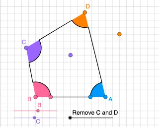
This GeoGebra example demonstrates how the interior angles of a quadrilateral can be constructed, measured, and related under geometric transformations. It focuses on angle construction using rays and segments, and on how rotation, translation, and dilation (together with vectors) update the position of relevant geometric features while enabling angle-tracking through dynamic geometry. The construction uses Point, Ray, and Segment to define vertices and sides, Angle to compute each interior angle, Line and Intersect to establish precise angle rays, and Polygon to represent the quadrilateral itself. Transformations are implemented with Rotate, Translate, Dilate, and Vector to generate the revamped configuration and to visualize angle changes/constraints. Additional objects such as Circle and CircleSector help illustrate geometric regions associated with the angles, while Min and CurveCartesian support organizing computed quantities and auxiliary geometry. Suitable for secondary-school geometry instruction and interactive lessons on angle concepts, quadrilateral properties, and transformation-based reasoning.
GeoGebra Commands & Parameters
Point(Ray[B + (1, 0), B + (2, 0)]) → ARotate(A, (a * π / 180), B) → A'Angle(A, B, A') → αRay(B, A') → fSegment(B, A) → gPoint(f) → CAngle(B, C, A) → βRotate(B, γ, C) → B'Angle(B, C, B') → δRay(C, B') → hPoint(h) → DRay(D, A) → iSegment(A, B) → jSegment(B, C) → kSegment(C, D) → lSegment(D, A) → mMin({j, k, l, m}) → bRay(A, B) → nRay(B, C) → pCircle(B, (0.3 * b)) → cIntersect(c, n, 2) → EIntersect(c, p, 1) → FCircle(C, (0.3 * b)) → dCircle(D, (0.3 * b)) → eCircle(A, (0.3 * b)) → qIntersect(d, h, 1) → GIntersect(d, p, 2) → HIntersect(e, i, 1) → IIntersect(e, h, 2) → JIntersect(q, n, 1) → KIntersect(q, i, 2) → LAngle(C, D, A) → εLine(B, A) → f_1Dilate(A, If[0 < u ≤ 1, 1 - u, 0], B) → A'_1Vector(A, A'_1) → vDilate(B, If[1 < u ≤ 2, 2 - u, 0], C) → B'_1Vector(B, B'_1) → wDilate(C, If[2 < u ≤ 3, 3 - u, 0], D) → C'Vector(C, C') → u_1Polygon(B, A, D, C) → poly1, b_1, a_1, d_2, c_2Intersect(c, n, 1) → MIntersect(c, p, 1) → NIntersect(d, p, 1) → OIntersect(d, h, 1) → PIntersect(e, h, 1) → QIntersect(e, i, 1) → RIntersect(q, i, 1) → SIntersect(q, n, 1) → TCircleSector(B, M, N) → rCircleSector(C, O, P) → sCircleSector(D, Q, R) → tCircleSector(A, S, T) → c_1Angle(B, C, D) → ζAngle(D, A, B) → ηCircle(V, (0.3 * b)) → d_1Circle(W, (0.3 * b)) → e_1Circle(Z, (0.3 * b)) → g_1Circle(A_1, (0.3 * b)) → h_1Point(d_1) → B_1Point(h_1) → C_1Rotate(B_1, α, V) → D_1Rotate(C_1, (-η), A_1) → E_1CircleSector(V, B_1, D_1) → k_1CircleSector(A_1, E_1, C_1) → p_1Segment(N, O) → i_1Segment(P, Q) → j_1Segment(R, S) → l_1Segment(T, M) → m_1Point(e_1) → UPoint(g_1) → F_1Line(Z, l_1) → n_1Ray(Z, F_1) → q_1Point(n_1) → G_1Angle(F_1, Z, G_1) → θDilate(D, If[0 < o_1 ≤ 1, 1 - o_1, 0], Z) → D'Vector(D, D') → v_1Translate(t, v_1) → t'Rotate(t', If[0 < o_1 ≤ 1, ((-o_1) * θ), (-θ)], D') → t''Dilate(C, If[1 < o_1 ≤ 2, 2 - o_1, 0], W) → C'_1Vector(C, C'_1) → w_1Translate(s, w_1) → s'Line(W, j_1) → r_1Point(r_1) → H_1Angle(H_1, W, U) → λRotate(s', If[1 < o_1 ≤ 2, ((o_1 - 1) * λ), λ], C'_1) → s'_1Point(s_1) → I_1Angle(D, C, I_1) → ιLine(C, D) → g_2Point(f_2) → J_1Angle(J_1, D, C) → κAngle(C, D, A) → μCurveCartesian(x(A) + ((0.3 * b) * cos(t)), y(A) + ((0.3 * b) * sin(t)), t, π - η, π) → a_2CurveCartesian(x(C) + ((0.3 * b) * cos(t)), y(C) + ((0.3 * b) * sin(t)), t, α + π, α + π + δ) → b_2CurveCartesian(x(B) + ((0.3 * b) * cos(t)), y(B) + ((0.3 * b) * sin(t)), t, 0, α) → t_1CurveCartesian(x(D) + ((0.3 * b) * cos(t)), y(D) + ((0.3 * b) * sin(t)), t, κ, κ + μ) → e_2
AI Drawing Prompt Reference
Draw a quadrilateral ABCD and observe the changes in its interior angles through transformations. Start by drawing circles with a radius of 0.3 times the side length centered at B, intersecting with sides AB, BC, CD, and DA to get points E, F, G, H, I, J, K, and L. Then, use rotations and dilations to adjust the positions of points A, B, C, and D, observing the changes in the interior angles. Finally, construct quadrilateral ABCD using these points and segments, and use arcs and circles to illustrate the geometric regions associated with the angles.
The prompt above was compiled from the original drawing commands and is for reference only.