
Visualizing Functions of Two Variables (Version 3)
Loading the math board and drawing, please wait…
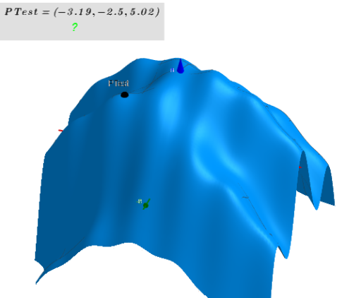
① This GeoGebra example demonstrates how to dynamically visualize a function of two variables z=f(x,y) by rendering its surface, contour lines, and related geometric quantities, providing an intuitive understanding of 3D function graphs. ② Core mathematical concepts include bivariate functions, surfaces, level curves (implicit curves), differential equations, volume, and frequency distribution, bridging calculus, analytic geometry, and applied mathematics. ③ Construction highlights: from the summary, commands such as Polygon, ImplicitCurve, IntersectPath, Locus, and PolyLine are used to build surfaces and paths; Sequence, Zip, Text, and Join generate dynamic text and sequences; sliders adjust parameters; Point, Vector, and Line create auxiliary elements; RemoveUndefined, Sum, and Length handle data and computations. ④ Suitable for high school to university-level mathematics instruction, especially for visualizing multivariable calculus, differential equations, and mathematical experiments, as well as for teachers creating interactive courseware.
GeoGebra Commands & Parameters
Polygon((x_{max}, y_{max}), (x_{min}, y_{max}), (x_{min}, y_{min}), (x_{max}, y_{min})) → VV, j, t, c, dIf(b_a, Nx_a, 1) → Nx1_aPolygon((x((ro; α)), y((ro; α)), z_{min}) + PTest, (x((ro; α + 180°)), y((ro; α + 180°)), z_{min}) + PTest, (x((ro; α + 180°)), y((ro; α + 180°)), z_{max}) + PTest, (x((ro; α)), y((ro; α)), z_{max}) + PTest) → poly1, k, l, m, pImplicitCurve(f(x, y) - f(x(C), y(C))) → ICurve_2IntersectPath(plane0, f(x, y)) → ICurve_3Point(ICurve_2) → R0Length(lr2) → llr2Sequence((x(Element[lr2, i]), y(Element[lr2, i]), f(x(Element[lr2, i]), y(Element[lr2, i]))), i, 1, llr2) → lllPmin01If(Length[lllPmin01] ≟ 0, false, true) → bwllPmin01Length(lr1) → llr1Sequence((x(Element[lr1, i]), y(Element[lr1, i]), f(x(Element[lr1, i]), y(Element[lr1, i]))), i, 1, llr1) → lllPmax01If(Length[lllPmax01] ≟ 0, false, true) → bwllPmax01If(bwllPmax01, Max[z(lllPmax01)], 1000) → Maxz0If(bwllPmax01, IndexOf[Maxz0, Sequence[z(Element[lllPmax01, i]), i, 1, Length[lllPmax01]]], 1000) → Indexmaxz0If(b, true, false) → hIf(h, Nx, 1) → Nx1Length(lr3) → llr3Point(Segment[(0, 0), (6.28319, 0)]) → AfPoint(Segment[Px2, Px1]) → AxPoint(Segment[Py2, Py1]) → AyTextfield(N_{V1}) → inputBox1Textfield(x_{min}) → inputBox2Textfield(x_{max}) → inputBox3Textfield(y_{min}) → inputBox4Textfield(y_{max}) → inputBox5Textfield(f) → inputBox6Textfield(z_{min}) → inputBox7Textfield(z_{max}) → inputBox8Point(Segment[Pz2, Pz1]) → AzTextfield(ω_c) → inputBox9Textfield(vt) → inputBox10Sum(Sequence[If[f(x(PTest), y(PTest)) - f(x(Element[lr01, i]), y(Element[lr01, i])) > 0, 1, 0], i, 1, n]) → ext1RotateText("z_{min}=" + z_{min} + "", 90°) → Text2RotateText("z_{max}=" + z_{max} + "", 90°) → Text6Sequence(Segment[Element[l0maxmin2, k], Element[l0maxmin2, k + 1]], k, 1, Length[l0maxmin2]) → linelmaxmin2Sequence(Element[lr1, i], i, 1, llr1) → lPmaxSequence(Element[lr2, i], i, 1, llr2) → lPminSequence(Element[lr3, i], i, 1, llr3) → lPsadIf(bwllPmin01, Min[z(lllPmin01)], 1000) → Minz0If(bwllPmin01, IndexOf[Minz0, Sequence[z(Element[lllPmin01, i]), i, 1, Length[lllPmin01]]], 1000) → Indexminz0Element(lr2, Indexminz0) → P_{min0}If(bwllPmin01, Element[lllPmin01, Indexminz0], (1000, 1000, 1000)) → zmin2Point(Liste1) → C111aLocus(C1110a, C111a) → locPolyLine(l0maxmin1) → linelmaxmin11If(bwllPmax01, Element[lllPmax01, Indexmaxz0], (1000, 1000, 1000)) → zmax2RemoveUndefined(Sequence[If[f(x(PTest), y(PTest)) - f(x(Element[lr01, i]), y(Element[lr01, i])) > 0, i, NaN], i, 1, n]) → lr04Zip(Vector[b, a], a, Sequence[Element[lr01, Element[lr04, i]], i, 1, Length[lr04]], b, Sequence[Element[lr02, Element[lr04, i]], i, 1, Length[lr04]]) → lr06Sequence((x(Element[lr01, i]), y(Element[lr01, i]), f(x(Element[lr01, i]), y(Element[lr01, i]))), i, 1, n) → lr013Sequence((x(Element[lr02, i]), y(Element[lr02, i]), f(x(Element[lr02, i]), y(Element[lr02, i]))), i, 1, n) → lr023Zip(Vector[b, a], a, Sequence[Element[lr013, Element[lr04, i]], i, 1, Length[lr04]], b, Sequence[Element[lr023, Element[lr04, i]], i, 1, Length[lr04]]) → lr063Zip(Vector[a, b], a, Sequence[Element[lr01, Element[lr05, i]], i, 1, Length[lr05]], b, Sequence[Element[lr02, Element[lr05, i]], i, 1, Length[lr05]]) → lr07Zip(Vector[a, b], a, Sequence[Element[lr013, Element[lr05, i]], i, 1, Length[lr05]], b, Sequence[Element[lr023, Element[lr05, i]], i, 1, Length[lr05]]) → lr073Textfield(zoom_{3D}) → InputBox1Element(lr1, rmax - 1) → PzmaxElement(lr2, rmin - 1) → PzminElement(lr3, rsad - 1) → PzsadText("( x , y , z )") → TextR01Join({{TextR01}, lllPmax01}) → llPmax01Element(lr1, Indexmaxz0) → P_{max0}Sequence((x(Element[lr3, i]), y(Element[lr3, i]), f(x(Element[lr3, i]), y(Element[lr3, i]))), i, 1, llr3) → lllPspJoin({{TextR01}, lllPmin01}) → llPmin01Join({{TextR01}, lllPsp}) → llPsad01Element(lllPsp, rsad - 1) → Pzsad_{3D}Element(lllPmax01, rmax - 1) → Pzmax_{3D}Element(lllPmin01, rmin - 1) → Pzmin_{3D}Textfield(A) → InputBox2RemoveUndefined(Sequence[If[f(x(PTest), y(PTest)) - f(x(Element[lr01, i]), y(Element[lr01, i])) > 0, i, (-i)], i, 1, n]) → lr04cAppend(lr04c, Element[lr04c, 1]) → lr04ccSum(Sequence[If[(Element[lr04cc, i] * Element[lr04cc, i + 1]) < 0, 1, 0], i, 1, n + 1]) → lr04cccLine(A, RoR) → iImplicitCurve(f(x, y) - zi) → list3ImplicitCurve(f(x, y) - zii) → list4Vector(R0, R41) → w_11Vector(R0, R0 + R11) → u_11Textfield(ω0_c) → InputBox3Textfield(r_a) → InputBox5Point(c) → GPoint(j) → HPoint(w_11, 1) → IVector(F, I_{3D}) → vIf(ext1 ≟ n, 1, If[ext1 ≟ 0, 2, If[lr04ccc > 2 ∧ lr04ccc ≤ 4, 3, 4]]) → rooTextfield(n_c) → InputBox6Textfield(a_c) → InputBox7Textfield(r_{lc}) → InputBox8Textfield(vt) → InputBox9PolyLine(Bl) → BlyPolyLine(Gr) → GryPolyLine(Ro) → RoyTextfield(Nx) → ResolutionTextfield(r) → InputBox11Textfield(v_{m4}) → InputBox4Textfield(Nz) → InputBox10Textfield(n) → InputBox12Textfield(rr) → InputBox13Textfield(r_{ext}) → InputBox14Textfield(v_{zi}) → InputBox15Textfield(d_1) → InputBox16Textfield(f_1) → InputBox17Textfield(v_{m3}) → InputBox18
AI Drawing Prompt Reference
Create a 3D plot of a bivariate function surface with contour lines, extreme points (maxima, minima, and saddle points), and cross-sectional curves along specified directions. Include a rectangular base region, adjustable sliders and input fields for function expression, coordinate ranges, and parameters. Highlight extreme points with distinct colors and display their numerical labels. Also show intersection curves with a plane and gradient vectors or trajectories from extreme points. The overall layout includes coordinate axes, grid, and dynamic text for interactive exploration.
The prompt above was compiled from the original drawing commands and is for reference only.