Level Curves of a Two-Variable Function

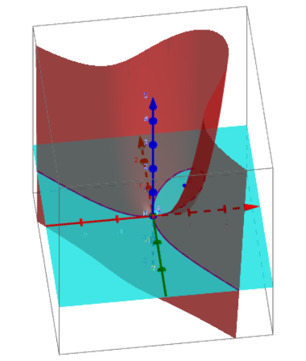
① This GeoGebra example dynamically displays the level curves (contour lines) of a two-variable function f(x,y), showing the family of curves where the function equals different constants k. ② The core mathematical concept is level curves in multivariable calculus, which help visualize horizontal slices of a surface, the direction of the gradient, and how function values change; it also involves ellipses and quadratic curves. ③ Construction highlights: from the summary, a slider k controls the contour height, the function f is defined, parameters a and b adjust the curve shape, points A and B and object g may represent auxiliary lines or gradients, the 'rastro' (trace) feature tracks moving points, and a button (botón1) triggers animation or reset, enabling dynamic observation of how level curves change with k. ④ Suitable for introductory university calculus or multivariable function courses, and also for advanced high school enrichment, providing an intuitive bridge from single-variable graphs to level sets, and preparing students for partial derivatives, gradients, and extrema.