
Visualizing Euclid's Algorithm by David Wees
Loading the math board and drawing, please wait…
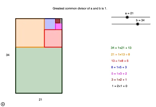
This example demonstrates the execution and geometric representation of Euclid's algorithm. It involves core math concepts like division, sequences, difference, and slope. Constructed using GeoGebra commands Min, Polygon, Midpoint, If, and objects such as a, b, A, scale, D, B, C. Suitable for high school mathematics teaching to help students intuitively understand the algorithm's principles and geometric significance.
GeoGebra Commands & Parameters
Min(5 / a, 5 / b) → scalePolygon(C, D, B, A) → q1, c, d, b_1, a_1Midpoint(C, A) → EMidpoint(B, A) → FMin(a, b) → s1If(a > b, (floor(a / s1) * s1), 0) → ss2aIf(b > a, (floor(b / s1) * s1), 0) → ss2bIf(a > b, a - s2, (s2 * ns2)) → ss3aIf(b > a, b - s2, (s2 * ns2)) → ss3bIf(b > a, Min[a - (s2 * ns2), s2], Min[b - (s2 * ns2), s2]) → s3If(b > a, (s1 * ns1) + (s3 * ns3), (s2 * ns2)) → ss4bIf(b > a, (s2 * ns2), (s1 * ns1) + (s3 * ns3)) → ss4aIf(b > a, (s2 * ns2) + (s4 * ns4), (s1 * ns1) + (s3 * ns3)) → ss5aIf(b > a, (s1 * ns1) + (s3 * ns3), (s2 * ns2) + (s4 * ns4)) → ss5bIf(b > a, (s2 * ns2) + (s4 * ns4), (s1 * ns1) + (s3 * ns3) + (s5 * ns5)) → ss6aIf(b > a, (s1 * ns1) + (s3 * ns3) + (s5 * ns5), (s2 * ns2) + (s4 * ns4)) → ss6bIf(b ≥ a, Sequence[Polygon[((m * scale), (ss4b * scale)), ((m * scale) + (s4 * scale), (ss4b * scale)), 4], m, ss4a, (s4 * (ns4 - 1)) + ss4a, s4], Sequence[Polygon[((ss4a * scale), (m * scale)), ((ss4a * scale) + (s4 * scale), (m * scale)), 4], m, ss4b, (s4 * (ns4 - 1)) + ss4b, s4]) → sequence4If(b ≥ a, Sequence[Polygon[((ss5a * scale), (m * scale)), ((ss5a * scale) + (s5 * scale), (m * scale)), 4], m, ss5b, (s5 * (ns5 - 1)) + ss5b, s5], Sequence[Polygon[((m * scale), (ss5b * scale)), ((m * scale) + (s5 * scale), (ss5b * scale)), 4], m, ss5a, (s5 * (ns5 - 1)) + ss5a, s5]) → sequence5If(b ≥ a, Sequence[Polygon[(0, (m * scale)), ((s1 * scale), (m * scale)), 4], m, 0, (s1 * (ns1 - 1)), s1], Sequence[Polygon[((m * scale) + (s1 * scale), 0), ((m * scale) + (s1 * scale), (s1 * scale)), 4], m, 0, (s1 * (ns1 - 1)), s1]) → sequence1If(b ≥ a, Sequence[Polygon[((m * scale), (ss2b * scale)), ((m * scale) + (s2 * scale), (ss2b * scale)), 4], m, 0, (s2 * (ns2 - 1)), s2], Sequence[Polygon[((ss2a * scale), (m * scale)), ((ss2a * scale) + (s2 * scale), (m * scale)), 4], m, 0, (s2 * (ns2 - 1)), s2]) → sequence2If(b ≥ a, Sequence[Polygon[((ss3a * scale), (m * scale)), ((ss3a * scale) + (s3 * scale), (m * scale)), 4], m, ss3b, (s3 * (ns3 - 1)) + ss3b, s3], Sequence[Polygon[((m * scale), (ss3b * scale)), ((m * scale) + (s3 * scale), (ss3b * scale)), 4], m, ss3a, (s3 * (ns3 - 1)) + ss3a, s3]) → sequence3If(b > a, (s2 * ns2) + (s4 * ns4) + (s6 * ns6), (s1 * ns1) + (s3 * ns3) + (s5 * ns5)) → ss7aIf(b > a, (s1 * ns1) + (s3 * ns3) + (s5 * ns5), (s2 * ns2) + (s4 * ns4) + (s6 * ns6)) → ss7bIf(b ≥ a, Sequence[Polygon[((ss7a * scale), (m * scale)), ((ss7a * scale) + (s7 * scale), (m * scale)), 4], m, ss7b, (s7 * (ns7 - 1)) + ss7b, s7], Sequence[Polygon[((m * scale), (ss7b * scale)), ((m * scale) + (s7 * scale), (ss7b * scale)), 4], m, ss7a, (s7 * (ns7 - 1)) + ss7a, s7]) → sequence7If(b ≥ a, Sequence[Polygon[((m * scale), (ss6b * scale)), ((m * scale) + (s6 * scale), (ss6b * scale)), 4], m, ss6a, (s6 * (ns6 - 1)) + ss6a, s6], Sequence[Polygon[((ss6a * scale), (m * scale)), ((ss6a * scale) + (s6 * scale), (m * scale)), 4], m, ss6b, (s6 * (ns6 - 1)) + ss6b, s6]) → sequence6
AI Drawing Prompt Reference
Create a geometric visualization of Euclid's algorithm. Start with a rectangle whose side lengths represent two positive integers, scaled appropriately. Inside this rectangle, fill it with a series of smaller squares or rectangles, each corresponding to the remainders obtained during the successive divisions. Arrange these blocks horizontally or vertically in a step-like or grid pattern, depending on which number is larger, to illustrate the iterative subtraction and remainder process. The final figure consists of multiple nested or adjacent rectangular regions, clearly showing how the algorithm reduces the dimensions until reaching the greatest common divisor.
The prompt above was compiled from the original drawing commands and is for reference only.