Visualizing a Function with No Limit at a Point

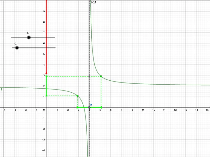
This example demonstrates how a function can fail to have a limit at a specific point, highlighting the divergent or path-dependent behavior as inputs approach that location. The key mathematical concepts include limits (including the idea of a limit not existing at a point), local behavior near singularities, and geometric interpretation connected to tangent-related constructions. Construction-wise, it uses GeoGebra primitives such as Point and Segment to define essential points and measurement segments, then builds a function object (f) together with parameter and auxiliary objects (e.g., a, alpha, g, A, B, C, D, h, i, E, F, j, k, l, BigA, p, and equation-related object eq1). These elements are arranged to generate a graph/surface-like visualization that captures what happens to the function near the target point via structured geometric relationships. Suitable for high school to early university learners studying calculus and mathematical analysis, and for classroom demonstrations and explorations of limit existence through dynamic geometry.