
Visualization of Independent Identically Distributed Random Variables
Loading the math board and drawing, please wait…
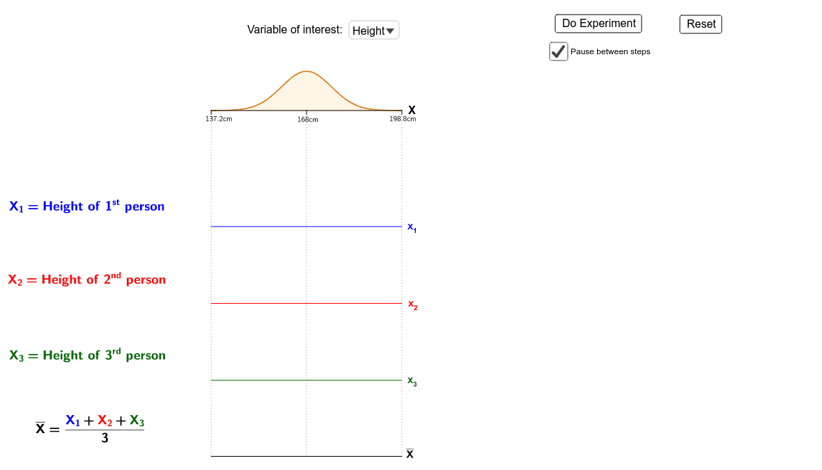
This applet visualizes the concept of independent identically distributed (i.i.d.) random variables. It covers core probability concepts such as probability density functions, sampling distributions, and the law of large numbers. Construction utilizes GeoGebra commands like Sequence for data generation, RandomUniform for simulation, and IntegralBetween for area calculation under curves. Objects include distribution curves and statistical data lists. Suitable for high school or college statistics courses to demonstrate theoretical distributions and empirical data convergence.
GeoGebra Commands & Parameters
Sequence(If[distribution ≟ 1, RandomNormal[0.5, 0.13], InverseGamma[α, β, RandomUniform[0, 1]]], i, 1, 1000) → datalist3rawSequence(If[distribution ≟ 1, RandomNormal[0.5, 0.13], InverseGamma[α, β, RandomUniform[0, 1]]], i, 1, 1000) → datalist2rawSequence(If[distribution ≟ 1, RandomNormal[0.5, 0.13], InverseGamma[α, β, RandomUniform[0, 1]]], i, 1, 1000) → datalist1rawZip((xx + yy + zz) / 3, xx, datalist1, yy, datalist2, zz, datalist3) → meanlistrawElement(datalist1, experiment) → x1activeIf(distribution ≟ 1, F1, F2) → FRandomUniform(4.5, F(x1active)) → y1Element(datalist2, experiment) → x2activeRandomUniform(4.5, F(x2active)) → y2Element(datalist3, experiment) → x3activeRandomUniform(4.5, F(x3active)) → y3Element(datalist3, 4) → x43Element(datalist3, 3) → x33Element(datalist3, 2) → x23Element(datalist3, 1) → x13Element(datalist2, 4) → x42Element(datalist2, 3) → x32Element(datalist2, 2) → x22Element(datalist2, 1) → x12Element(datalist1, 4) → x41Element(datalist1, 3) → x31Element(datalist1, 2) → x21Element(datalist1, 1) → x11Element(meanlist, 1) → m1Element(meanlist, 2) → m2If(distribution ≟ 1, ((x - 0.5) / 0.13 * 8) + 168, (x * 100)) → scalefuncIf(distribution ≟ 1, "cm", "k") → unitsElement({x11dp, x21dp, x31dp, x41dp}, experiment) → x1dpactiveElement({x12dp, x22dp, x32dp, x42dp}, experiment) → x2dpactiveElement({x13dp, x23dp, x33dp, x43dp}, experiment) → x3dpactiveElement(meanlist, 3) → m3Element(meanlist, 4) → m4Element({m1dp, m2dp, m3dp, m4dp}, experiment) → mdpactiveTranslate(DotPlot[Take[datalist2, 1, experiment], false, 0.006], (0, 2 + dpscale / 2)) → datalist2_{dp}underlayerTranslate(DotPlot[Take[datalist1, 1, experiment], false, 0.006], (0, 3 + dpscale / 2)) → datalist1_{dp}underlayerTranslate(DotPlot[Take[datalist3, 1, experiment], false, 0.006], (0, 1 + dpscale / 2)) → datalist3_{dp}underlayerSegment((0, 4.5), (1, 4.5)) → aIntegralBetween(4.5, F, 0, 1, false) → cSegment((0, 0), (1, 0)) → maxisIf(distribution ≟ 1, "", "\$") → dollarsTranslate(F, (0, (-1.5 * t51))) → x1FTranslate(F, (0, (-2.5 * t51))) → x2FTranslate(F, (0, (-3.5 * t51))) → x3FIf(distribution ≟ 1, M1, M2) → MSegment((0, 4.5), (0, 4.45)) → tick1Segment((1, 4.5), (1, 4.45)) → tick3Segment((0.5, 4.5), (0.5, 4.45)) → tick2Segment((0, 2.99), (1, 2.99)) → x1axisSegment((0, 1.99), (1, 1.99)) → x2axisSegment((0, 0.99), (1, 0.99)) → x3axisTranslate(DotPlot[Take[meanlist, 1, experiment], false, 0.006], (0, dpscale / 2)) → Mean_{dp}Segment((0, 4.5), (0, 0)) → guideline1Segment((1, 4.5), (1, 0)) → guideline2Segment((0.5, 4.5), (0.5, 0)) → guideline3