Gaussian Success: Visualizing Normal Distribution and Limits

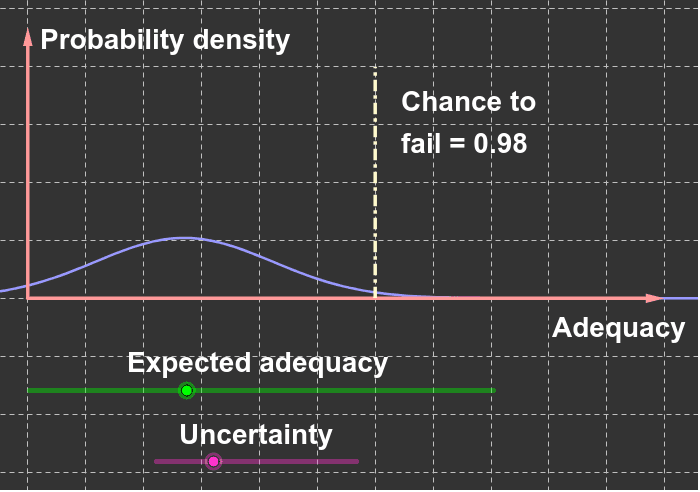
① This GeoGebra example dynamically illustrates the Gaussian (normal) distribution curve and its associated geometric constructions, showing how the probability density function changes with parameters and approaches limits. ② Core mathematical concepts include normal distribution, variance, limits, upper and lower sums (Riemann sums), coordinates, and ratios, bridging abstract statistical ideas with visual geometry. ③ Construction details: using commands such as Point, Vector, Segment, Function, and Intersect, with objects E, A, b, B, v, D, e, a, d, F, C, and multiple text labels (text1_1 to text1_5) to annotate key values and relationships; sliders or parameters likely control the curve's shape. ④ Suitable for high school to undergraduate courses in probability, statistics, and calculus, ideal for demonstrating properties of the normal distribution, limit concepts, or Riemann sum approximations, fostering intuitive understanding.