
Variety of Shapes for a Quartic
Loading the math board and drawing, please wait…
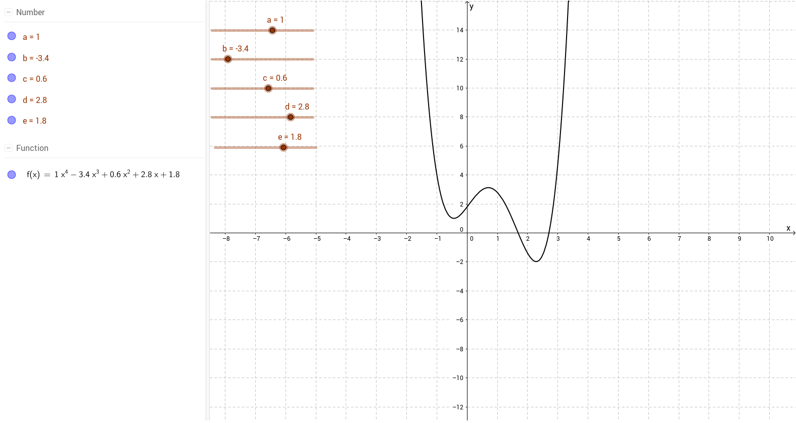
This example demonstrates the diverse shapes possible for quartic equations (fourth-degree polynomial equations) in three-dimensional space. It involves core math concepts like coordinate geometry, function graphing, parametric equations, and surface shape analysis. The construction uses GeoGebra objects a, b, c, d, e, f, likely as parameters controlling the equation's coefficients or form. Suitable for high school and above students to understand the geometric meaning and variety of high-degree polynomial surfaces.
GeoGebra Commands & Parameters
Numeric a(1.0)Numeric b(-3.4)Numeric c(0.6)Numeric d(2.8)Numeric e(1.8)f(x) = (a * x^(4)) + (b * x^(3)) + (c * x^(2)) + (d * x) + e
AI Drawing Prompt Reference
Please draw a graph of a quartic polynomial function in three-dimensional space. The function is controlled by parameters a, b, c, d, e, f, with the form f(x) = a*x^4 + b*x^3 + c*x^2 + d*x + e. Show the diversity of shapes for different parameter values, including surfaces and curves. Based on coordinate geometry, function graphing, and parametric equations, present the geometric meaning of high-degree polynomial surfaces. Ensure the graph is clear, with parameter values such as a=1.0, b=-3.4, c=0.6, d=2.8, e=1.8.
The prompt above was compiled from the original drawing commands and is for reference only.