
Using Correlation Coefficient to Describe Data Relationship Strength
Loading the math board and drawing, please wait…
In collections
AP Statistics
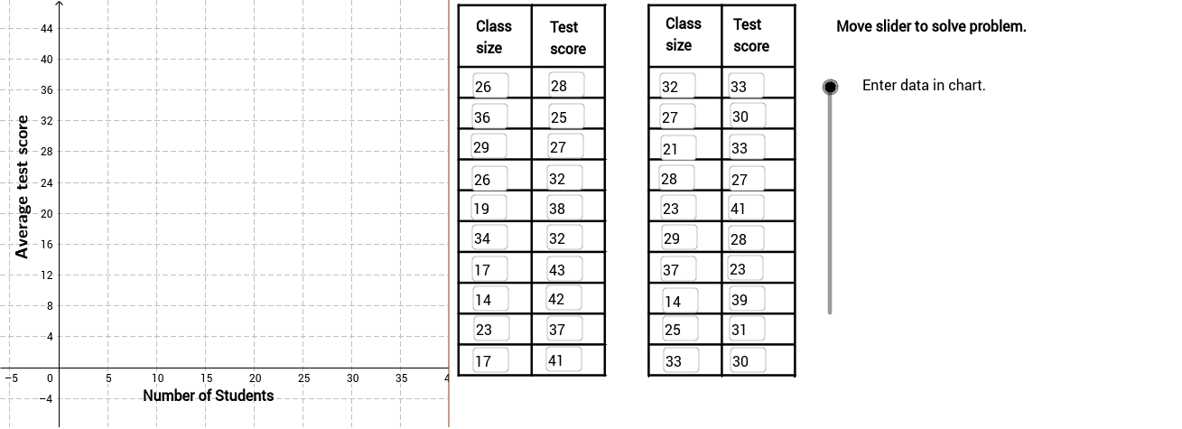
This GeoGebra example demonstrates how to fit a line to a scatter plot and compute the Pearson product-moment correlation coefficient (PMCC) to quantitatively describe the strength of the linear relationship between two data sets. Core mathematical concepts include correlation coefficient, linear regression, scatter plots, and strength-of-association interpretation. The construction employs GeoGebra commands such as FitLineY for the regression line, PMCC for the correlation value, Textfield and If for dynamic conditional text, and Polygon, Sequence, Segment, and RotateText for plotting data points, drawing segments, and labeling objects A1 through B19. Suitable for high school statistics and probability courses or introductory college statistics, supporting classroom demonstration and self-paced inquiry into how correlation coefficient values correspond to data scatter tightness.
GeoGebra Commands & Parameters
FitLineY(PointList1) → LineFitPMCC(PointList1) → CorCoeffTextfield(A2) → InA2Textfield(A3) → InA3Textfield(A4) → InA4Textfield(A5) → InA5Textfield(A6) → InA6Textfield(A7) → InA7Textfield(A8) → InA8Textfield(A9) → InA9Textfield(A10) → InA10Textfield(A11) → InA11Textfield(A12) → InA12Textfield(A13) → InA13Textfield(A14) → InA14Textfield(A15) → InA15Textfield(A16) → InA16Textfield(A17) → InA17Textfield(A18) → InA18Textfield(A19) → InA19Textfield(A20) → InA20Textfield(A21) → InA21Textfield(B2) → InB2Textfield(B3) → InB3Textfield(B4) → InB4Textfield(B5) → InB5Textfield(B6) → InB6Textfield(B7) → InB7Textfield(B8) → InB8Textfield(B9) → InB9Textfield(B10) → InB10Textfield(B11) → InB11Textfield(B12) → InB12Textfield(B13) → InB13Textfield(B14) → InB14Textfield(B15) → InB15Textfield(B16) → InB16Textfield(B17) → InB17Textfield(B18) → InB18Textfield(B19) → InB19Textfield(B20) → InB20Textfield(B21) → InB21If(CorVisible, "Hide Correlation Coefficient", "Show Correlation Coefficient") → CorButtonIf(LineVisible, "Hide Best Fit Line", "Show Best Fit Line") → LineButtonPolygon((40, y(Corner[1])), Corner[2], Corner[3], (40, y(Corner[4]))) → poly1, a, b, c, dSequence(Segment[(41, -1 + 4 * i), (56, -1 + 4 * i)], i, 0, 10) → Linesh1Sequence(Segment[(41 + 7.5 * i, -1), (41 + 7.5 * i, 47)], i, 0, 2) → Linesv1Sequence(Segment[(60.5 + 7.5 * i, -1), (60.5 + 7.5 * i, 47)], i, 0, 2) → Linesv2Sequence(Segment[(60.5, -1 + 4 * i), (75.4, -1 + 4 * i)], i, 0, 10) → Linesh2Segment((41, 47), (56, 47)) → top1Segment((60.5, 47), (75.5, 47)) → top2RotateText("Average test score", 90*°) → SideLegend
AI Drawing Prompt Reference
Draw a coordinate plane with a grid background, plot about twenty data points forming a scatter plot, automatically fit a best‑fit regression line through the points, display the Pearson correlation coefficient value on the chart, and add two toggle buttons to show or hide the correlation coefficient and the regression line; keep the design clean for statistics teaching demonstrations in a clear visual style.
The prompt above was compiled from the original drawing commands and is for reference only.