
Unrolling the Unit Circle: A Geometric View of Trigonometry
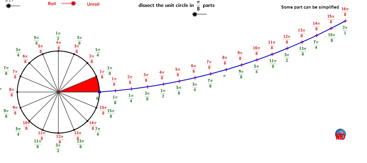
Loading the math board and drawing, please wait…
This example uses a dynamic construction to “unroll” the unit circle, visually mapping an angle parameter on the circle to a corresponding unfolded geometric representation. It helps learners understand why sine and cosine are determined by unit-circle coordinates, bridging circular motion with a linear/unfolded perspective. Key concepts include the unit circle, central angles and radians, the geometric meaning of sin/cos, and the use of arc/sector shapes to relate circular and unfolded measurements. The construction employs GeoGebra commands such as Min, Sequence, Zip, and Element to generate and access parameterized point sequences; Segment, Midpoint, and OrthogonalLine to build guiding lines and perpendiculars; Circle, CircleArc, and CircleSector to create the circle, arcs, and sectors; PolyLine to draw the unfolded path; and Angle to label/compute the central angle. It is intended for high-school to early undergraduate students and is well-suited for classroom demonstrations and self-study on trigonometry and radian-based geometry.
GeoGebra Commands & Parameters
Min(Max[betaRegularized(2, 2.3, Extend), 0.0001], 0.9999) → Animat1Sequence(A + (i, 0), i, R, R) → PointdebutZip(Circle[C, B], B, Pointdebut) → CerclesZip(Rotate[B, ((((360 * ° / (((2 * Radius[K]) * π))) * 2) * Distance[A, B]) * π), C], K, Cercles, B, Pointdebut) → PointFinsElement(PointFins, Length[PointFins]) → B'Segment(B, B') → bMidpoint(B, B') → DOrthogonalLine(D, b) → cCircle(A, R) → aSegment(A, B') → gSegment(B, B') → hSequence(Rotate[B, i, A], i, 0, 6.283185307179586, π / m) → liste1PolyLine(Append[B, PointFins]) → ABSCircleArc(C, B, B') → dAngle(B, C, B') → αSequence(Rotate[B, i, C], i, 0, α, α / ((2 * m))) → liste2Sequence(Segment[A, Element[liste1, i]], i, 1, Length[liste1]) → liste4Sequence(Text[k - 1 + "π/" + m, Element[liste2, k] - (0.1, 0.2)], k, 1, (2 * m) + 1) → liste3Sequence(Text["" + (k) + " π / " + m, A - (0.15, 0) + (R + 0.15; (k * π / m))], k, 2, (2 * m) - 1, 2) → liste5CircleSector(A, B, Element[liste1, 2]) → eSequence(Text["\frac{" + (k) + ((π * "}{")) + m + "}", A - (0.085, -0.12) + (R + 0.145; (k * π / m)), true, true], k, 1, (2 * m) - 1) → l2Sequence(Text["\frac{" + (k) + ((π * "}{")) + m + "}", Element[liste2, k + 1] - (0.125, -0.35), true, true], k, 1, (2 * m)) → l2bSequence(Text[If[i ≟ 0, "0", If[i ≟ m, "π", "\frac{" + (i / GCD[i, m]) + ((π * "}{") + (m / GCD[i, m]) + "}")]], liste2(i + 1) - (0.1, 0.1), true, true], i, 0, (2 * m)) → l1Sequence(Text[If[i ≟ 0, "0", If[i ≟ m, " π", "\frac{" + (i / GCD[i, m]) + ((π * "}{") + (m / GCD[i, m]) + "}")]], A - (0.1, -0.125) + (R + 0.365; (i * π / m)), true, true], i, 1, (2 * m) - 1) → l1b
AI Drawing Prompt Reference
Draw a unit circle and show its 'unrolling' process to explain trigonometric functions. Start from a point on the circle, move along the circumference, and unroll it into a straight line to show the correspondence between angles and unfolded lengths. Use concentric circles and sectors to represent angle divisions, and label the angle values and trigonometric function values on the unrolled line to help understand the connection between circular motion and linear unfolding.
The prompt above was compiled from the original drawing commands and is for reference only.