
Unit Circle and Sine Graph Dynamic Visualization
Loading the math board and drawing, please wait…
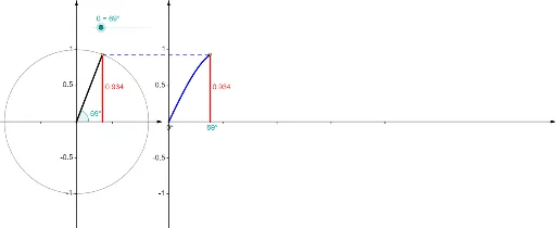
This example dynamically links the unit circle to the sine function graph, showing how the angle on the circle corresponds to the sine value on the curve. It demonstrates the geometric definition of sine as the y-coordinate of a point on the unit circle, and how this maps to the periodic sine wave. Core concepts include the unit circle, trigonometric functions (sine), angle measurement in radians, function graphing, and periodicity. The construction uses GeoGebra commands such as Point, Rotate, Angle, Function, Segment, Circle, Vector, and Sequence, creating objects like the unit circle, rotating angle θ, sine function f, and auxiliary points (P, A', Q) to trace the relationship. A slider controls the angle, updating the corresponding point on the sine curve in real time. This is ideal for high school trigonometry, pre-calculus, or introductory calculus courses, helping students bridge geometric intuition and functional representation.
GeoGebra Commands & Parameters
Point(Ray[(0, 0), (-1, 0)]) → BRotate(A, θ, B) → PRotate(A, θ, B) → A'Angle(A, B, A') → αRotate(A, θ, B) → A'_1Angle(A, B, A'_1) → βFunction(sin((120° * x)), 0, x(Q)) → fSegment(Q, (x(Q), 0)) → eCircle(B, A) → cSegment(B, P) → aVector((x(B), y(Corner[1])), (x(B), y(Corner[4]))) → uVector((0, y(Corner[1])), (0, y(Corner[4]))) → wVector((0, 0), (x(Corner[2]), 0)) → zSequence(Segment[((0.75 * i), 0), ((0.75 * i), -0.025)], i, 1, 4) → list1Segment(P, (x(P), 0)) → bVector(B - (1.2, 0), B + (1.2, 0)) → vSequence(Segment[(0, (0.5 * i) - 1), (-0.025, (0.5 * i) - 1)], i, 0, 4) → list2Sequence(Segment[(x(B), (0.5 * i) - 1), (x(B) - 0.025, (0.5 * i) - 1)], i, 0, 4) → list3Segment(P, Q) → dSequence(Segment[B + ((0.5 * i) - 1, 0), B + ((0.5 * i) - 1, -0.025)], i, 0, 4) → list4Point(Ray[(0, 0), (-1, 0)]) → B_1Rotate(A_1, θ, B_1) → P_1Rotate(A_1, θ, B_1) → A'_2Rotate(A_1, θ, B_1) → A'_3Circle(B_1, A_1) → c_1Segment(B_1, P_1) → a_1
AI Drawing Prompt Reference
Draw a unit circle and dynamically plot an angle θ on the circle, corresponding to point P. Rotate point A to get point P, then draw line segment a connecting P to the center B. Simultaneously, plot a sine function graph f with domain from 0 to x(Q). Connect point P to the origin along the x-axis to form line segment e. Use rotation and angle measurement to demonstrate the relationship between angle θ and the sine value.
The prompt above was compiled from the original drawing commands and is for reference only.