
Unit Circle and Tangent Graph
Loading the math board and drawing, please wait…
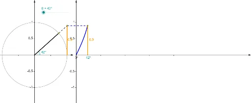
This example demonstrates the geometric relationship between the unit circle and the tangent function graph. It involves core math concepts like the unit circle, trigonometric functions, tangent function, angles, and slopes. Construction highlights include using GeoGebra commands such as Point, Rotate, Segment, Angle, Vector, Sequence, and Function. Suitable for high school mathematics teaching to understand the generation and properties of trigonometric function graphs.
GeoGebra Commands & Parameters
Point(Ray[(0, 0), (-1, 0)]) → BRotate(A, θ, B) → PSegment(A, Intersect[Line[B, P], x = x(A)]) → hSegment(P, Intersect[Line[B, P], x = x(A)]) → gRotate(A, θ, B) → A'Angle(A, B, A') → αRotate(A, θ, B) → A'_1Angle(A, B, A'_1) → βSegment(Q, (x(Q), 0)) → eCircle(B, A) → cSegment(B, P) → aVector((x(B), y(Corner[1])), (x(B), y(Corner[4]))) → uVector((0, y(Corner[1])), (0, y(Corner[4]))) → wVector((0, 0), (x(Corner[2]), 0)) → zSequence(Segment[((0.75 * i), 0), ((0.75 * i), -0.025)], i, 1, 4) → list1Vector(B - (1.2, 0), B + (1.2, 0)) → vSequence(Segment[(0, (0.5 * i) - 1), (-0.025, (0.5 * i) - 1)], i, 0, 4) → list2Sequence(Segment[(x(B), (0.5 * i) - 1), (x(B) - 0.025, (0.5 * i) - 1)], i, 0, 4) → list3Sequence(Segment[B + ((0.5 * i) - 1, 0), B + ((0.5 * i) - 1, -0.025)], i, 0, 4) → list4Segment(C, Q) → dFunction(tan((120° * x)), 0, (θ / ((360 * γ)) * 3)) → fPoint(Ray[(0, 0), (-1, 0)]) → B_1Rotate(A_1, θ, B_1) → P_1Rotate(A_1, θ, B_1) → A'_2Rotate(A_1, θ, B_1) → A'_3Circle(B_1, A_1) → c_1