
Unit Circle and Sine Graph by Sam Waterfield
Loading the math board and drawing, please wait…
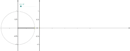
This example dynamically demonstrates the correlation between a point on the unit circle and its corresponding sine value, visually illustrating the formation of the sine curve. Core math concepts include the unit circle, trigonometric functions, coordinate geometry, and the relationship between angles and function graphs. Construction highlights involve GeoGebra commands such as Point, Rotate, Angle, Function, Segment, Circle, Vector, and Sequence. It is suitable for high school mathematics education, helping students understand the origin and properties of trigonometric function graphs and enhancing spatial reasoning skills.
GeoGebra Commands & Parameters
Point(Ray[(0, 0), (-1, 0)]) → BRotate(A, θ, B) → PRotate(A, θ, B) → A'Angle(A, B, A') → αRotate(A, θ, B) → A'_1Angle(A, B, A'_1) → βFunction(sin((120° * x)), 0, x(Q)) → fSegment(Q, (x(Q), 0)) → eCircle(B, A) → cSegment(B, P) → aVector((x(B), y(Corner[1])), (x(B), y(Corner[4]))) → uVector((0, y(Corner[1])), (0, y(Corner[4]))) → wVector((0, 0), (x(Corner[2]), 0)) → zSequence(Segment[((0.75 * i), 0), ((0.75 * i), -0.025)], i, 1, 4) → list1Segment(P, (x(P), 0)) → bVector(B - (1.2, 0), B + (1.2, 0)) → vSequence(Segment[(0, (0.5 * i) - 1), (-0.025, (0.5 * i) - 1)], i, 0, 4) → list2Sequence(Segment[(x(B), (0.5 * i) - 1), (x(B) - 0.025, (0.5 * i) - 1)], i, 0, 4) → list3Segment(P, Q) → dSequence(Segment[B + ((0.5 * i) - 1, 0), B + ((0.5 * i) - 1, -0.025)], i, 0, 4) → list4Point(Ray[(0, 0), (-1, 0)]) → B_1Rotate(A_1, θ, B_1) → P_1Rotate(A_1, θ, B_1) → A'_2Rotate(A_1, θ, B_1) → A'_3Circle(B_1, A_1) → c_1Segment(B_1, P_1) → a_1