
Underdamping Simulation: Spring-Mass System Dynamics
Loading the math board and drawing, please wait…
In collections
MATH1052-edX
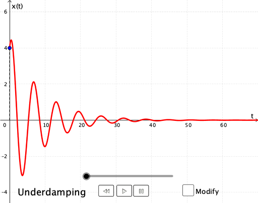
This GeoGebra example demonstrates the underdamped oscillation of a spring-mass system, showing how displacement decays over time with a sinusoidal pattern. The core mathematical concepts involve second-order ordinary differential equations (SolveODE), damping coefficient β, natural frequency ω, initial conditions (position x0 and velocity xprime0), and the exponential decay envelope. Construction highlights: the SolveODE command solves the equation of motion; functions like Length, First, Zip, Max, Min process the solution curve; Segment, Ray, and CurveCartesian draw the spring, platform, and displacement graph; interactive Textfield and Button controls allow adjusting parameters (mass m, damping β, stiffness k) with real-time updates. Suitable for high school physics or introductory university mechanics courses, this example aids in teaching vibrations, differential equations, and parameter sensitivity analysis.
GeoGebra Commands & Parameters
SolveODE((2 * p), ω^(2), 0, 0, x0, xprime0, maxTime, 0.04) → SolutionLength(Solution) → lenFirst(Solution, len) → LPIf(D < 0, "Underdamping", If[D ≟ 0, "Critical damping", "Overdamping"]) → textClassZip(y(P), P, LP) → LxPMax(LxP) → maxMin(LxP) → minSegment(C1, C2) → platformTextfield(x0) → Inpx0Textfield(xprime0) → Inpxprime0Textfield(m) → InpmTextfield(k) → InpkTextfield(β) → InpβRay((100, 0), (-100, 0)) → eqposIf(ylength < 0, CurveCartesian[(width * sin((((fr * 2) * π) * (t - y_1) / (y_0 - y_1)))) + x(A2), t, t, y_0, y_1], CurveCartesian[(width * sin((((fr * 2) * π) * (t - y_1) / (y_0 - y_1)))) + x(A2), t, t, y_1, y_0]) → springCurveCartesian((width * sin((((fr * 2) * π) * (t - sect) / (y_0 - sect)))) + x(A2), t, t, sect, y_0) → springFixedSegment(PS, PS + (0, sect)) → endSegment((x(A2), 0), (x(A2), 0) + (0, sect)) → endFixedIf(abs(max) < 0.4, 0.5, max) → ymaxIf(abs(min) < 0.4, -1.2, min) → yminSegment((0, ftime), ((facTime * time), ftime)) → horSegment(((facTime * time), 0), ((facTime * time), ftime)) → verTextfield(maxTime) → InpMTime
AI Drawing Prompt Reference
Draw a spring-mass system showing underdamped oscillation. Start by drawing a platform, then attach a spring to it, with the other end connected to a mass. The mass oscillates underdamped on the platform, with amplitude decaying over time. Use sliders to adjust mass, spring stiffness, and damping coefficient, updating the graph in real-time. Include the displacement curve of the mass, showing maximum and minimum displacement, and time markers on the timeline.
The prompt above was compiled from the original drawing commands and is for reference only.