
Two Uniform Points on a Sphere from One Uniform Distribution: Cube V=8
Loading the math board and drawing, please wait…
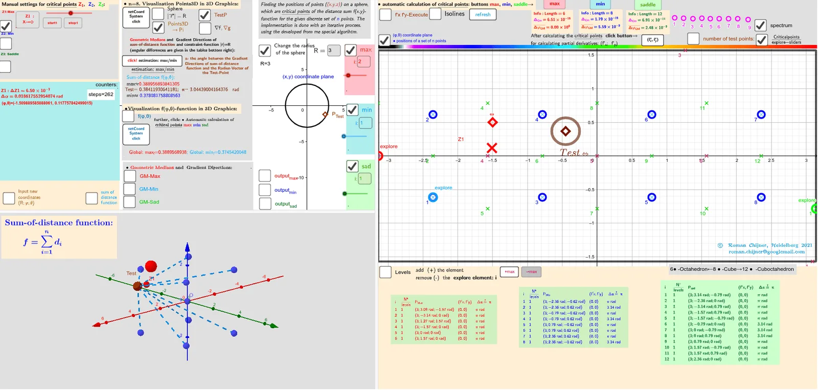
This example demonstrates how to generate two different points that are uniformly distributed on a sphere using a single uniform source (e.g., one uniform random parameter mapped through geometry). It visualizes the construction and highlights how uniformity is achieved on the spherical surface rather than inside a volume. Key mathematics includes solid geometry on the sphere, uniform probability on a manifold (sphere surface), vector geometry, angle/length-based relationships, and constrained selection using min/max logic. The GeoGebra construction uses Sphere and Circle to define the spherical setting and relevant regions; PointIn, Polygon, and Vector to form candidate constructions and determine membership; Angle and Length to compute spatial relations between points; Function with If as well as Max/Min to implement the piecewise mapping/feasibility constraints tied to the “Cube V=8” volume-normalization idea; and Zip/Flatten with TableText and Textfield to structure computed outputs. It also employs CurveCartesian for plotting and labels/annotations (RotateText, arrow) to clarify key quantities. Suitable for advanced high-school through early university learners in probability & sampling, geometry construction, and mathematical visualization (Monte Carlo style).
GeoGebra Commands & Parameters
Function(f01, (-π), π, ((-π)) / 2, π / 2) → f0Zip((x(a), y(a), f0(a)), a, Zmin_2) → fmin3DZip((x(a), y(a), f0(a)), a, Zmax_2) → fmax3DVector((1.3 * Z3), (1.5 * Z3)) → AVZ3rVector((1.3 * Z3), (1.3 * Z3) + UnitVector[Sum[Zip[UnitVector[a - Z3], a, lP]]]) → AVZ3Polygon({((-π), ((-π)) / 2), ((-π), π / 2), (π, π / 2), (π, ((-π)) / 2)}) → q_2PointIn(q_2) → Atest_2Vector((1.3 * Z2), (1.5 * Z2)) → AVZ2rVector((1.3 * Z2), (1.3 * Z2) + UnitVector[Sum[Zip[UnitVector[a - Z2], a, lP]]]) → AVZ2Vector((1.3 * Z1), (1.5 * Z1)) → AVZ1rVector((1.3 * Z1), (1.3 * Z1) + UnitVector[Sum[Zip[UnitVector[a - Z1], a, lP]]]) → AVZ1Vector((1.3 * Atest_R), (1.3 * Atest_R) + UnitVector[Sum[Zip[UnitVector[a - Atest_R], a, lP]]]) → AVtestVector((1.3 * Atest_R), (1.5 * Atest_R)) → AVtestrSphere(O, R) → spheraCircle(O, R, xOyPlane) → cPointIn(q_2) → RZ1_2PointIn(q_2) → RZ2_2Angle(AVtest, AVtestr) → αAAngle(AVZ1, AVZ1r) → αZ1Angle(AVZ2, AVZ2r) → αZ2Zip(Segment[Atest_R, p], p, lP) → segSum(seg) → sum_segPolyLine({((-π), ((-π)) / 2), ((-π), π / 2), (π, π / 2), (π, ((-π)) / 2), ((-π), ((-π)) / 2)}) → q1Flatten(Sequence[Sequence[((-π) + ((2 * π / na) * i), ((-π)) / 2 + (π / na * j)), j, 1, na], i, 1, na]) → ltest_2Zip((R; x(a); y(a)), a, ltest_2) → ltest_3Length(lZmax') → lälZmax'Textfield(n) → InputBox11alfa(R, lP, lZsad') → αsadIf(αZ1 > 100°, 180° - αZ1, αZ1) → αZ1'Textfield(m_1) → InputBox12Textfield(t) → InputBox13Textfield(m_2) → InputBox14PointIn(q_2) → RZ3_2Sum(Zip[1 / Length[p - Z3], p, lP]) → ZahZ3Angle(AVZ3, AVZ3r) → αZ3Textfield(R) → InputBox1Textfield(na) → InputBox2Max(f(Zmax_2)) → max_fMin(f(Zmin_2)) → min_fZip(Text["d_{" + (a) + "}", (Atest_R + Element[lP, a]) / 2], a, 1…n) → lPtxtZip(Segment[F_o, p], p, lP) → seg0Sum(seg0) → sum_seg0RotateText(txt, 90°) → txt1Sum(lZ3sad) → sumlZ3sadTextfield(Points3D) → InputBox7Textfield(lZsad') → InputBox17Textfield(lZmin') → InputBox16Textfield(lZmax') → InputBox15Textfield(jmin) → InputBox18Textfield(jmax) → InputBox19Textfield(jsad) → InputBox20Zip(Text["" + (b), a - (0.1, 0.1)], a, Zmax_2, b, 1…Length[Zmax_2]) → l2maxtxtZip(Text["" + (b), a - (0.1, 0.1)], a, Zmin_2, b, 1…Length[Zmin_2]) → l2mintxtZip(Text["" + (b), a - (0.1, 0.1)], a, Zsad_2, b, 1…Length[Zsad_2]) → l2sadtxtZip(Vector[r1, (1.153846154 * r1)], r1, (1.3 * Zip[(R * UnitVector[a]), a, lZmax'])) → lVmaxrZip(Vector[r1, (1.153846154 * r1)], r1, (1.3 * Zip[(R * UnitVector[a]), a, lZmin'])) → lVminrZip(Vector[r1, (1.153846154 * r1)], r1, (1.3 * Zip[(R * UnitVector[a]), a, lZsad'])) → lVsadralfa(R, lP, lZmax') → αmaxalfa(R, lP, lZmin') → αminarrow(R, lP, lZmax') → lVmaxarrow(R, lP, lZmin') → lVminarrow(R, lP, lZsad') → lVsadCurveCartesian((-π) + ((2 * π) * a), ((-π)) / 2, f0((-π) + ((2 * π) * a), ((-π)) / 2), a, 0, 1) → par1CurveCartesian((-π) + ((2 * π) * a), π / 2, f0((-π) + ((2 * π) * a), π / 2), a, 0, 1) → par2CurveCartesian((-π), ((-π)) / 2 + (π * a), f0((-π), ((-π)) / 2 + (π * a)), a, 0, 1) → par3CurveCartesian(π, ((-π)) / 2 + (π * a), f0(π, ((-π)) / 2 + (π * a)), a, 0, 1) → par4Polygon({((-π), ((-π)) / 2), ((-π), π / 2), (π, π / 2), (π, ((-π)) / 2)}) → q_3Zip((x(a), y(a), f0(a)), a, Zsad_2) → fsad3DTextfield(achs) → InputBox3Zip(Atest_2 + (0.2; ((2 * π / 10) * k)), k, 0…9) → l0rSum(Unique[sgn(f(Atest_2) - f(l0r))]) → sum_rSum(Sequence[If[sum00_r(i) ≠ sum00_r(i + 1), 1, 0], i, 1, Length[sum00_r] - 1]) → sum01_rCircle(Atest_2, 0.2) → ciTableText(Append["i", Sequence[Length[lZsad']]], Append["\frac{N°}{levels} ", msad], Append["P_{sad }", lZsad'], Append["(f'x,f'y)", lZf'xysad], Append[" Δα≟ π ", αsad], "v") → text2cTableText(Append["i", Sequence[Length[αmax]]], Append["\frac{N°}{levels} ", mmax], Append["P_{Max }", lZmax'], Append["(f'x,f'y)", lZf'xymax], Append[" Δα≟ π ", αmax], "v") → text2aTableText(Append["i", Sequence[Length[αmin]]], Append["\frac{N°}{levels} ", mmin], Append["P_{Min }", lZmin'], Append["(f'x,f'y)", lZf'xymin], Append[" Δα≟ π ", αmin], "v") → text2b
AI Drawing Prompt Reference
Generate two uniformly distributed points on a sphere to demonstrate how a single uniform distribution source can be mapped to the spherical surface. Use a sphere and a circle to define the space, calculate the relationships between points using angles and lengths, and apply vector geometry with conditional logic (like min/max) for point selection and distribution. Start by drawing the sphere and reference circle, then create two vectors representing candidate points, compute their angular relationships with the sphere, and finally adjust the vectors based on conditions to ensure the points are uniformly distributed on the sphere.
The prompt above was compiled from the original drawing commands and is for reference only.