
Two distinct uniform points on a sphere from one uniform distribution via a regu
Loading the math board and drawing, please wait…
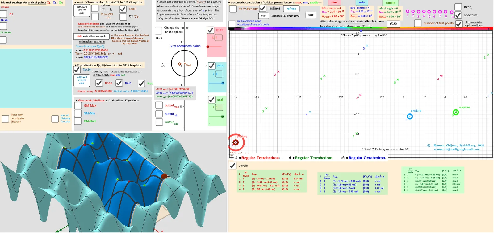
This example demonstrates how to generate two different points on a sphere that are uniformly distributed, using only a single underlying uniform random source, with a regular tetrahedron (with parameter V=4) providing the construction that controls how the two points differ while preserving uniformity on the sphere. Key concepts include spherical geometry, vectors, rotation/angle relations, and probability-style uniform sampling constraints on a curved surface. The construction uses GeoGebra commands and objects such as Sphere and Circle to define the spherical setting and auxiliary geometry, PointIn to test membership in relevant regions, Vector and Angle to build directional relationships, RotateText and PolyLine/Polygon to visualize transformations and the geometric structure, and If together with Max/Min and Length to enforce selection/feasibility conditions for the second point. It also employs Textfield/TableText to display computed parameters (e.g., angles/thresholds and bounds like Zmin/Zmax, fmin3D/fmax3D) and CurveCartesian to plot verification curves associated with the constraints. Suitable for high school through early university learners studying geometry, computational modeling, and probability-inspired sampling on manifolds, and for GeoGebra-based demonstrations of spherical uniformity checks.
GeoGebra Commands & Parameters
Polygon({((-π), ((-π)) / 2), ((-π), π / 2), (π, π / 2), (π, ((-π)) / 2)}) → q_2PointIn(q_2) → Atest_2Function(f01, (-π), π, ((-π)) / 2, π / 2) → f0Zip((x(a), y(a), f0(a)), a, Zmin_2) → fmin3DZip((x(a), y(a), f0(a)), a, Zmax_2) → fmax3DVector((1.3 * Z3), (1.5 * Z3)) → AVZ3rVector((1.3 * Z3), (1.3 * Z3) + UnitVector[Sum[Zip[UnitVector[a - Z3], a, lP]]]) → AVZ3Vector((1.3 * Z2), (1.5 * Z2)) → AVZ2rVector((1.3 * Z2), (1.3 * Z2) + UnitVector[Sum[Zip[UnitVector[a - Z2], a, lP]]]) → AVZ2Vector((1.3 * Z1), (1.5 * Z1)) → AVZ1rVector((1.3 * Z1), (1.3 * Z1) + UnitVector[Sum[Zip[UnitVector[a - Z1], a, lP]]]) → AVZ1Vector((1.3 * Atest_R), (1.3 * Atest_R) + UnitVector[Sum[Zip[UnitVector[a - Atest_R], a, lP]]]) → AVtestVector((1.3 * Atest_R), (1.5 * Atest_R)) → AVtestrSphere(O, R) → spheraCircle(O, R, xOyPlane) → cPointIn(q_2) → RZ1_2PointIn(q_2) → RZ2_2Angle(AVtest, AVtestr) → αAAngle(AVZ1, AVZ1r) → αZ1Angle(AVZ2, AVZ2r) → αZ2Zip(Segment[Atest_R, p], p, lP) → segSum(seg) → sum_segPolyLine({((-π), ((-π)) / 2), ((-π), π / 2), (π, π / 2), (π, ((-π)) / 2), ((-π), ((-π)) / 2)}) → q1Flatten(Sequence[Sequence[((-π) + ((2 * π / na) * i), ((-π)) / 2 + (π / na * j)), j, 1, na], i, 1, na]) → ltest_2Zip((R; x(a); y(a)), a, ltest_2) → ltest_3Length(lZmax') → lälZmax'Textfield(n) → InputBox11alfa(R, lP, lZsad') → αsadIf(αZ1 > 100°, 180° - αZ1, αZ1) → αZ1'Textfield(m_1) → InputBox12Textfield(t) → InputBox13Textfield(m_2) → InputBox14PointIn(q_2) → RZ3_2Sum(Zip[1 / Length[p - Z3], p, lP]) → ZahZ3Angle(AVZ3, AVZ3r) → αZ3Textfield(R) → InputBox1Textfield(na) → InputBox2Max(f(Zmax_2)) → max_fMin(f(Zmin_2)) → min_fZip(Text["d_{" + (a) + "}", (Atest_R + Element[lP, a]) / 2], a, 1…n) → lPtxtZip(Segment[F_o, p], p, lP) → seg0Sum(seg0) → sum_seg0RotateText(txt, 90°) → txt1Sum(lZ3sad) → sumlZ3sadTextfield(Points3D) → InputBox7Textfield(lZsad') → InputBox17Textfield(lZmin') → InputBox16Textfield(lZmax') → InputBox15Textfield(jmin) → InputBox18Textfield(jmax) → InputBox19Textfield(jsad) → InputBox20Zip(Text["" + (b), a - (0.1, 0.1)], a, Zmax_2, b, 1…Length[Zmax_2]) → l2maxtxtZip(Text["" + (b), a - (0.1, 0.1)], a, Zmin_2, b, 1…Length[Zmin_2]) → l2mintxtZip(Text["" + (b), a - (0.1, 0.1)], a, Zsad_2, b, 1…Length[Zsad_2]) → l2sadtxtZip(Vector[r1, (1.153846154 * r1)], r1, (1.3 * Zip[(R * UnitVector[a]), a, lZmax'])) → lVmaxrZip(Vector[r1, (1.153846154 * r1)], r1, (1.3 * Zip[(R * UnitVector[a]), a, lZmin'])) → lVminrZip(Vector[r1, (1.153846154 * r1)], r1, (1.3 * Zip[(R * UnitVector[a]), a, lZsad'])) → lVsadralfa(R, lP, lZmax') → αmaxalfa(R, lP, lZmin') → αminarrow(R, lP, lZmax') → lVmaxarrow(R, lP, lZmin') → lVminarrow(R, lP, lZsad') → lVsadCurveCartesian((-π) + ((2 * π) * a), ((-π)) / 2, f0((-π) + ((2 * π) * a), ((-π)) / 2), a, 0, 1) → par1CurveCartesian((-π) + ((2 * π) * a), π / 2, f0((-π) + ((2 * π) * a), π / 2), a, 0, 1) → par2CurveCartesian((-π), ((-π)) / 2 + (π * a), f0((-π), ((-π)) / 2 + (π * a)), a, 0, 1) → par3CurveCartesian(π, ((-π)) / 2 + (π * a), f0(π, ((-π)) / 2 + (π * a)), a, 0, 1) → par4Polygon({((-π), ((-π)) / 2), ((-π), π / 2), (π, π / 2), (π, ((-π)) / 2)}) → q_3Textfield(achs) → InputBox3Circle(Atest_2, 0.2) → ciTableText(Append["i", Sequence[Length[lZsad']]], Append["\frac{N°}{levels} ", msad], Append["P_{sad }", lZsad'], Append["(f'x,f'y)", lZf'xysad], Append[" Δα≟ π ", αsad], "v") → text2cTableText(Append["i", Sequence[Length[αmax]]], Append["\frac{N°}{levels} ", mmax], Append["P_{Max }", lZmax'], Append["(f'x,f'y)", lZf'xymax], Append[" Δα≟ π ", αmax], "v") → text2aTableText(Append["i", Sequence[Length[αmin]]], Append["\frac{N°}{levels} ", mmin], Append["P_{Min }", lZmin'], Append["(f'x,f'y)", lZf'xymin], Append[" Δα≟ π ", αmin], "v") → text2bZip((x(a), y(a), f0(a)), a, Zsad_2) → fsad3DZip(Atest_2 + (r_c; ((2 * π / n_c) * k)), k, 0…(n_c - 1)) → l0rSum(Sequence[If[sum00_r(i) ≠ sum00_r(i + 1), 1, 0], i, 1, Length[sum00_r] - 1]) → sum01_rSum(Unique[sgn(f(Atest_2) - f(l0r))]) → sum_r
AI Drawing Prompt Reference
Draw a 3D sphere with a common center and radius, then visualize its parameter-domain boundaries using planar closed polylines. In the base plane (the plane containing the sphere’s defining circle), plot a quadrilateral outline corresponding to fixed angle ranges, and also draw a second quadrilateral outline with subdivided boundary points for verification. Choose a reference point whose direction lies inside the first closed region, then construct another direction on the sphere by enforcing the relation between the reference vector and a transformed/rotated direction so that the angle between them can be measured. Include angle annotations for the constructed directional pairs and indicate the constrained feasible regions relative to the drawn boundaries.
The prompt above was compiled from the original drawing commands and is for reference only.