
Trigonometric Function Transformation Example
Loading the math board and drawing, please wait…
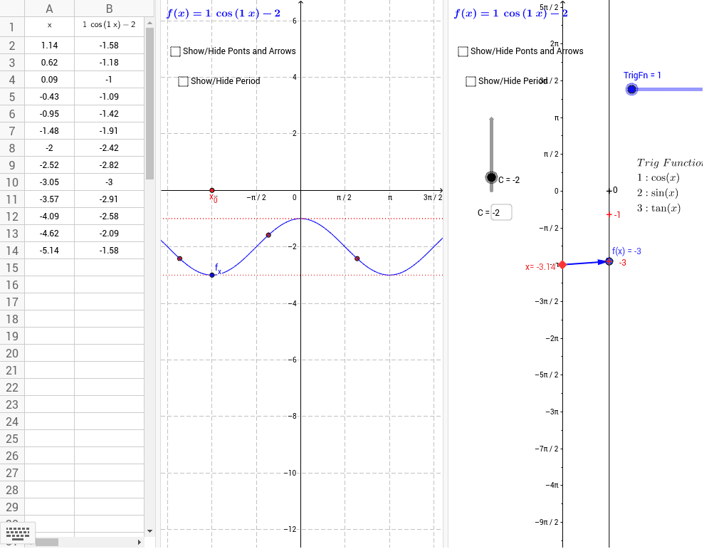
This example demonstrates the transformation of trigonometric functions, showing the basic properties and transformation rules of trigonometric functions. Using GeoGebra commands, dynamic observation of the changes in trigonometric function graphs can be achieved. The construction summary mentions the use of Element, Point, Vector, Segment, Sequence, Textfield, Derivative, Zip, etc. It is suitable for high school mathematics teaching and learning of trigonometric function transformations.
GeoGebra Commands & Parameters
Element(TrigL, TrigFn) → fPoint(yAxis) → aVector(a, f_a) → uSegment(C_1, D) → eVector(E, F) → vSequence((k, f(k)), k, C - π, C + π, 0.5235987755982988) → list1Sequence(Vector[(0, k), (2, f(k))], k, C - π, C + π, 0.5235987755982988) → list2Sequence(Segment[(i, f(i)), ((2 * C) - i, f((2 * C) - i))], i, C - π, C, 0.5235987755982988) → list3Vector(G, H) → wSegment(f_x, J) → jSequence(Segment[(i, f(i)), (π - i, f(π - i))], i, 0, 3.141592653589793, 0.5235987755982988) → suplTextfield(B) → inputBox1Textfield(C) → InputBox1Derivative(f) → f'Vector(f_a, (2, y(f_a) + f'(y(a)))) → hSequence(-5, 5) → nlistZip(((1 / B * ((2 * k) + 1)) * π / 2) - C / B, k, nlist) → xtrslistZip((z, f(z)), z, xtrslist) → xtrsptsZip(((1 / B * k) * π) - C / B, k, nlist) → xrtclistZip((z, f(z)), z, xrtclist) → xtrcptsTextfield(A) → InputBox2Segment(a, Q) → lSegment(a, P) → mVector(P, f_a) → nVector(Q, f_a) → pSegment(f_x, M) → sSegment(f_x, R) → q