
Triangle Trigonometry and Circle Geometry Demo
Loading the math board and drawing, please wait…
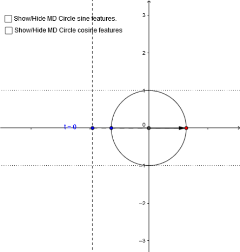
This example dynamically demonstrates the geometric relationship between a triangle's incircle and its sides and angles, visually showcasing the connection between trigonometric functions and circles. Core concepts include trigonometry, incircle, angles, vectors, and sequences. Construction highlights use of GeoGebra commands like Intersect, Point, Circle, Segment, Angle, OrthogonalLine, CircleArc, Vector, Sequence, and Zip. Suitable for high school mathematics education to understand the intrinsic link between trigonometric functions and geometric figures, enhancing spatial reasoning.
GeoGebra Commands & Parameters
Intersect(xAxis, yAxis) → APoint(yAxis) → ECircle(A, B) → cSegment(A, C) → aSegment(B, A) → bAngle(B, A, C) → αOrthogonalLine(C, yAxis) → dIntersect(d, yAxis) → DCircleArc(A, B, C) → eVector(C, D) → uVector(E, F) → vSegment(D, A) → hSegment(H, B) → iVector(t, C) → wOrthogonalLine(C, b) → jIntersect(j, i) → IVector(C, I) → zVector(E, K) → lSequence(n, n, -10, 10) → kZip((0, (((4 * j) + 1) * π / 2)), j, k) → sinmaxlZip((0, (((4 * j) - 1) * π / 2)), j, k) → sinminlZip(Segment[(0, (((4 * j) - 1) * π / 2)), (0, (((4 * j) + 1) * π / 2))], j, k) → sininclZip(Segment[(0, (((4 * j) + 1) * π / 2)), (0, (((4 * j) + 3) * π / 2))], j, k) → sindeclZip(Segment[(-1.5, (((4 * j) - 1) * π / 2)), (-1.5, (((4 * j) + 1) * π / 2))], j, k) → sininclcirZip(Segment[(-1.5, (((4 * j) + 1) * π / 2)), (-1.5, (((4 * j) + 3) * π / 2))], j, k) → sindeclcirVector(I, J) → mZip((0, ((2 * j) * π)), j, k) → cosmaxlZip((0, (((2 * j) - 1) * π)), j, k) → cosminlZip(Segment[(0, (((2 * j) - 1) * π)), (0, ((2 * j) * π))], j, k) → cosinclZip(Segment[(0, ((2 * j) * π)), (0, (((2 * j) + 1) * π))], j, k) → cosdeclZip(Segment[(-1.5, (((2 * j) - 1) * π)), (-1.5, ((2 * j) * π))], j, k) → cosinclcirZip(Segment[(-1.5, ((2 * j) * π)), (-1.5, (((2 * j) + 1) * π))], j, k) → cosdeclcir