
Three-Parameter Transformations of the Octahedron and Extreme Distributions
Loading the math board and drawing, please wait…
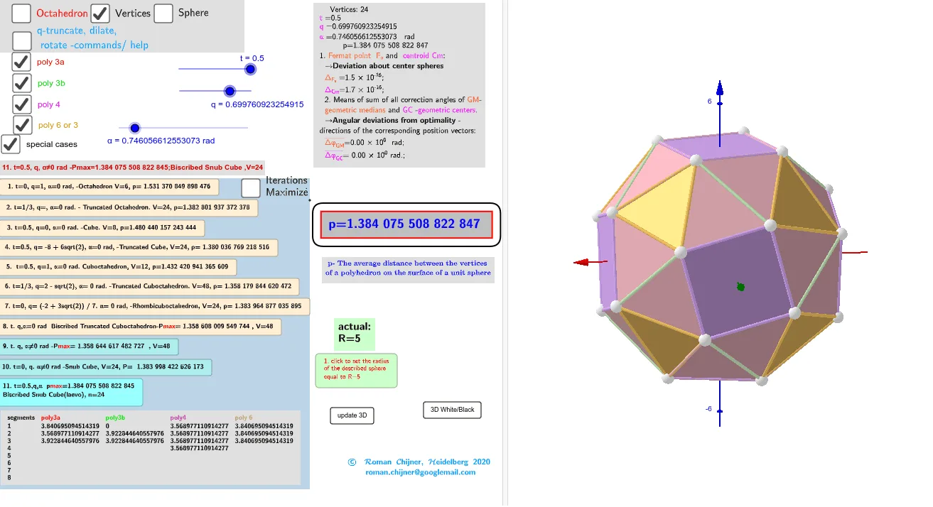
This example demonstrates the three-parameter transformations of the octahedron and their extreme distributions. Key mathematical concepts include transformations, extrema, and distributions. Using GeoGebra commands such as Length, Sequence, and Zip, you can dynamically adjust parameters to observe the transformation effects. Suitable for high school mathematics education and research.
GeoGebra Commands & Parameters
Length(m00(1)) → n00_1Length(m00) → n00Sequence({V00(m00(i, 1) + 1), V00(m00(i, 2) + 1), V00(m00(i, 3) + 1)}, i, 1, n00) → V00'Sequence(Dilate[Flatten[Sequence[V00'(i, j) + ((If[j < n00_1, V00'(i, j + 1), V00'(i, 1)] - V00'(i, j)) * {t, 1 - t}), j, 1, n00_1]], q, Cmi(i)], i, 1, n00) → V0aZip(Rotate[a, α, Line[(0, 0), b]], a, V0a, b, Cmi) → V0bJoin(V0b) → V0cIf(t ≟ 0 ∨ t ≟ 0.5 ∨ q ≟ 1 ∨ q ≟ 0, Unique[V0c], V0c) → V0ccLength(V0cc) → läV'Sequence(Polygon[Sequence[V00(m00(i, k) + 1), k, 1, Length[m00(1)]]], i, 1, Length[m00]) → Poly3Length(V0c) → läV0cSequence(Segment[V0c(m4(1, j)), V0c(m4(1, If[j ≟ 4, 1, j + 1]))], j, 1, 4) → seg4_iSequence(Segment[V0c(m6(1, j)), V0c(m6(1, If[j ≟ 6, 1, j + 1]))], j, 1, 6) → seg6_iSequence(Segment[V0c(m8(1, j)), V0c(m8(1, If[j ≟ 10, 1, j + 1]))], j, 1, 10) → seg8_iLength(V0cc) → n3Length(V00(1)) → läV00_1Sequence(Segment[V0c(m6a(1, j)), V0c(m6a(1, If[j ≟ 6, 1, j + 1]))], j, 1, 6) → seg6a_iKeepIf(x > 0, seg6_i) → seg6_i1KeepIf(x > 0, seg6a_i) → seg6a_i1KeepIf(x > 0, seg4_i) → seg4_i1KeepIf(x > 0, seg8_i) → seg8_i1Length(V0c(1)) → läV0c_1Dilate(q0, q, Cmi(1)) → q0'Sphere(O, läV0c_1) → spheSequence(Polygon[Sequence[V0c(m6(i, k)), k, 1, Length[m6(1)]]], i, 1, Length[m6]) → Poly6Sequence(Polygon[Sequence[V0c(m8(i, k)), k, 1, Length[m8(1)]]], i, 1, Length[m8]) → Poly8Sequence(Polygon[Sequence[V0c(m3a(i, k)), k, 1, Length[m3a(1)]]], i, 1, Length[m3a]) → Poly3aSequence(Polygon[Sequence[V0c(m3b(i, k)), k, 1, Length[m3b(1)]]], i, 1, Length[m3b]) → Poly3bSequence(Polygon[Sequence[V0c(m6a(i, k)), k, 1, Length[m6a(1)]]], i, 1, Length[m6a]) → Poly6aSequence(Polygon[Sequence[V0c(m4(i, k)), k, 1, Length[m4(1)]]], i, 1, Length[m4]) → Poly4Sequence(Polygon[Sequence[V0c(m4a(i, k)), k, 1, Length[m4a(1)]]], i, 1, Length[m4a]) → Poly4aSequence(Segment[V0c(m3a(1, j)), V0c(m3a(1, If[j ≟ 3, 1, j + 1]))], j, 1, 3) → seg3a_iSequence(Segment[V0c(m3b(1, j)), V0c(m3b(1, If[j ≟ 3, 1, j + 1]))], j, 1, 3) → seg3b_iSequence(Segment[V0c(m4a(1, j)), V0c(m4a(1, If[j ≟ 4, 1, j + 1]))], j, 1, 4) → seg4a_iKeepIf(x > 0, seg4a_i) → seg4a_i1TableText(Append["segments", 1…8], Append["\fgcolor{red}{ poly3a} ", seg3a_i], Append["\fgcolor{green}{poly3b}", seg3b_i], Append["\fgcolor{#BD33A4}{poly4}", seg4a_i1], Append["\fgcolor{#C19A6B}{poly\; 6\; }", seg6_i1], "v") → text6cTableText(Append["segments", 1…8], Append["\fgcolor{red}{ poly4} ", seg4_i1], Append["\fgcolor{green}{poly\; 6\; or\; 3}", seg6_i1], Append["\fgcolor{#C19A6B}{poly\; 8\; or\; 4}", seg8_i1], "v") → text6bText("" + p) → txt_pSum(Flatten[Sequence[Append[Sequence[Element[txt_p, i], i, m1(k), m2(k)], " "], k, 1, 5]]) → txtUm1Text(text18r, A, false, true) → text18s
AI Drawing Prompt Reference
Draw a three-parameter transformation of an octahedron, showing its extreme distributions. Start by constructing an octahedron, then adjust parameters using length and sequence commands to observe transformation effects. Dilate and rotate the transformed vertices to form new geometric shapes. Finally, label the edges and faces of the new shapes with different colors and add text annotations to compare the before and after transformations.
The prompt above was compiled from the original drawing commands and is for reference only.