
Three-Parameter Model Transformations of the Icosahedron with Extreme Distributi
Loading the math board and drawing, please wait…
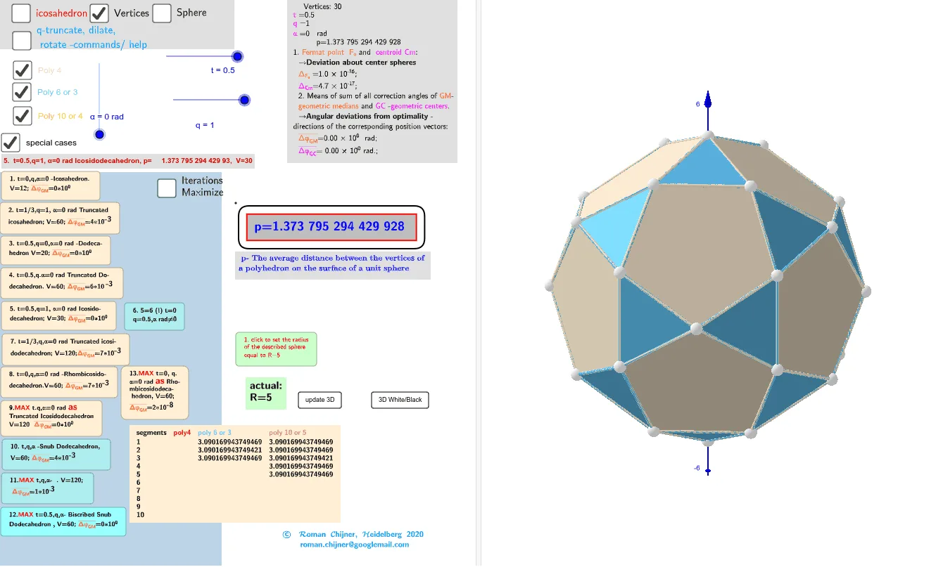
This example demonstrates the extreme distributions of an icosahedron under three-parameter model transformations. Key mathematical concepts include transformations, extreme distributions, and solid geometry. Using GeoGebra commands such as Length, Sequence, and Zip, the transformed icosahedron and its extreme distributions can be constructed. Suitable for high school mathematics education and research.
GeoGebra Commands & Parameters
Length(m00(1)) → n00_1Length(m00) → n00Sequence({V00(m00(i, 1) + 1), V00(m00(i, 2) + 1), V00(m00(i, 3) + 1)}, i, 1, n00) → V00'Sequence(Dilate[Flatten[Sequence[V00'(i, j) + ((If[j < n00_1, V00'(i, j + 1), V00'(i, 1)] - V00'(i, j)) * {t, 1 - t}), j, 1, n00_1]], q, Cmi(i)], i, 1, n00) → V0aZip(Rotate[a, α, Line[(0, 0), b]], a, V0a, b, Cmi) → V0bJoin(V0b) → V0cIf(t ≟ 0 ∨ t ≟ 0.5 ∨ q ≟ 1 ∨ q ≟ 0, Unique[V0c], V0c) → V0ccLength(V0cc) → läV'Sequence(Polygon[Sequence[V00(m00(i, k) + 1), k, 1, Length[m00(1)]]], i, 1, Length[m00]) → Poly3Length(V0c) → läV0cSequence(Segment[V0c(m4(1, j)), V0c(m4(1, If[j ≟ 4, 1, j + 1]))], j, 1, 4) → seg4_iSequence(Segment[V0c(m6(1, j)), V0c(m6(1, If[j ≟ 6, 1, j + 1]))], j, 1, 6) → seg6_iSequence(Segment[V0c(m10(1, j)), V0c(m10(1, If[j ≟ 10, 1, j + 1]))], j, 1, 10) → seg10_iLength(V0cc) → n3Length(V00(1)) → läV00_1Sequence(Segment[V0c(m3a(1, j)), V0c(m3a(1, If[j ≟ 3, 1, j + 1]))], j, 1, 3) → seg3a_iSequence(Segment[V0c(m3b(1, j)), V0c(m3b(1, If[j ≟ 3, 1, j + 1]))], j, 1, 3) → seg3b_iSequence(Segment[V0c(m5a(1, j)), V0c(m5a(1, If[j ≟ 5, 1, j + 1]))], j, 1, 5) → seg5a_iKeepIf(x > 0, seg6_i) → seg6_i1KeepIf(x > 0, seg4_i) → seg4_i1KeepIf(x > 0, seg10_i) → seg10_i1Length(V0c(1)) → läV0c_1Dilate(q0, q, Cmi(1)) → q0'Sphere(O, läV0c_1) → spheSequence(Polygon[Sequence[V0c(m6(i, k)), k, 1, Length[m6(1)]]], i, 1, Length[m6]) → Poly6Sequence(Polygon[Sequence[V0c(m10(i, k)), k, 1, Length[m10(1)]]], i, 1, Length[m10]) → Poly10Sequence(Polygon[Sequence[V0c(m3a(i, k)), k, 1, Length[m3a(1)]]], i, 1, Length[m3a]) → Poly3aSequence(Polygon[Sequence[V0c(m3b(i, k)), k, 1, Length[m3b(1)]]], i, 1, Length[m3b]) → Poly3bSequence(Polygon[Sequence[V0c(m5a(i, k)), k, 1, Length[m5a(1)]]], i, 1, Length[m5a]) → Poly5aSequence(Polygon[Sequence[V0c(m4(i, k)), k, 1, Length[m4(1)]]], i, 1, Length[m4]) → Poly4TableText(Append["segments", 1…6], Append["\fgcolor{#FE6F5E}{ poly3a} ", seg3a_i], Append["\fgcolor{#D19FE8}{ poly3b} ", seg3b_i], Append["\fgcolor{#008000}{poly\; 5\; }", seg5a_i], Append["\fgcolor{#008B8B}{poly\;6\; or\; 3 }", seg6_i1], "v") → text6cText("" + p) → txt_pSum(Flatten[Sequence[Append[Sequence[Element[txt_p, i], i, m1(k), m2(k)], " "], k, 1, 5]]) → txtUm1Text(text18r, A, false, true) → text18sTableText(Append["segments", 1…10], Append["\fgcolor{red}{ poly4} ", seg4_i1], Append["\fgcolor{#66CCFF}{poly\; 6\; or\; 3}", seg6_i1], Append["\fgcolor{#C19A6B}{poly\; 10\; or\; 5}", seg10_i1], "v") → text6b