
The Riemann Integral: Mapping Diagram and Graph
Loading the math board and drawing, please wait…
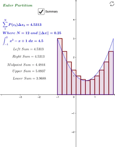
This example demonstrates the construction of a mapping diagram and graph for the Riemann integral. Key math concepts include the Riemann integral, function graphs, partitioning intervals, and summation approximations. GeoGebra commands/objects used in the construction summary are Sequence, Join, Take, Zip, If, Textfield, Integral, TrapezoidalSum, Sum, Max, Vector, and TableText. It is suitable for high school and above students studying calculus to visually understand the geometric meaning and calculation methods of integrals.
GeoGebra Commands & Parameters
Sequence(1, N) → N1LJoin({{a}, Sort[RandomUniform[a, b, N - 1]], {b}}) → randPartTake(randPart, 2, N + 1) → randPRTake(randPart, 1, N) → randPLZip(r - l, r, randPR, l, randPL) → h_kZip(a + (k * Δx), k, N1L) → ERx_kIf(ER ≟ 2, randPR, ERx_k) → Rx_kZip(a + ((k - 1) * Δx), k, N1L) → ELx_kIf(ER ≟ 2, randPL, ELx_k) → Lx_kZip(x(Max[f_p, A, B]), A, Lx_k, B, Rx_k) → fmax_kSequence(0, N) → N0LZip(a + (k * Δx), k, N0L) → EPartZip(y(Max[f_p, A, B]), A, Lx_k, B, Rx_k) → fmax_1Zip(y(Min[f_p, A, B]), A, Lx_k, B, Rx_k) → fmin_1Zip(RandomUniform[A, B], A, Lx_k, B, Rx_k) → randx_kIf(me ≟ 1, fLx_k, If[me ≟ 2, fRx_k, If[me ≟ 3, fMidx_k, If[me ≟ 4, fmax_1, If[me ≟ 5, fmin_1, franx_k]]]]) → fx_kIf(ER ≟ 1, EfΔx_k, randfΔx_k) → fΔx_kTextfield(f_p) → inputBox1If(ER ≟ 1, EPart, randPart) → x_kZip((0, t), t, x_k) → x_kMDZip((1, Sum[fΔx_k, j]), j, N1L) → Sumpts1Textfield(a) → inputBox2Textfield(b) → inputBox3If(ER ≟ 1, UpperSum[f_p, a, b, N], Sum[(fmax_1 * h_k)]) → UpSumIntegral(f_p, a, b) → IntegralIf(ER ≟ 1, LowerSum[f_p, a, b, N], Sum[(fmin_1 * h_k)]) → LowSumTrapezoidalSum(f_p, a, b, N) → TrapSumIf(ER ≟ 1, Sum[fmidΔx], Sum[(fMidx_k * h_k)]) → MdptSumSum(fΔx_k) → IntSumZip(x(Min[f_p, A, B]), A, Lx_k, B, Rx_k) → fmin_kIf(me ≟ 1, Lx_k, If[me ≟ 2, Rx_k, If[me ≟ 3, Midx_k, If[me ≟ 4, fmax_k, If[me ≟ 5, fmin_k, randx_k]]]]) → x'_kTextfield(a) → inputBox2_1Textfield(b) → inputBox3_1Zip((0, t), t, x'_k) → c_kMDZip(Vector[A, B], A, (0, Rx_k), B, Sumpts1) → SumarrowMax(h_k) → meshIntegral(f_p) → intPVector(Element[x_kMD, N + 1], Element[Sumpts1, N]) → f_{arrowb}Join({{(1, 0)}, Take[Sumpts1, 1, N - 1]}) → Sumpts2Zip(Vector[A, B], A, Sumpts2, B, Sumpts1) → dy_kMDVector(A, Targ0) → uZip(Polygon[(s, 0), (s, u), (t, u), (t, 0)], s, Lx_k, t, Rx_k, u, fx_k) → RectsIf(ER ≟ 1, "Euler", "Riemann") → ERTextIf(ER ≟ 1, Sum[(fRx_k * Δx)], Sum[(fRx_k * h_k)]) → RtSumIf(ER ≟ 1, LeftSum[f_p, a, b, N], Sum[(fLx_k * h_k)]) → LSumTableText({Join[{{"c_k"}, x'_k}], Join[{{"P(c_k)"}, fx_k}], Join[{{"P(c_k)Δx"}, fΔx_k}]}, "|_ccv") → TableTTextfield(N) → InputBox1
AI Drawing Prompt Reference
Draw the Riemann integral graph of a function f(x) over the interval [a, b]. Start by plotting the function and the interval partition lines. Then, calculate the upper and lower sums, and the trapezoidal sum. Next, draw rectangles for each subinterval and connect their tops to form the sum's graphical representation. Finally, show the integral value and the sum approximations.
The prompt above was compiled from the original drawing commands and is for reference only.