Tangent Planes and Linear Approximations Example

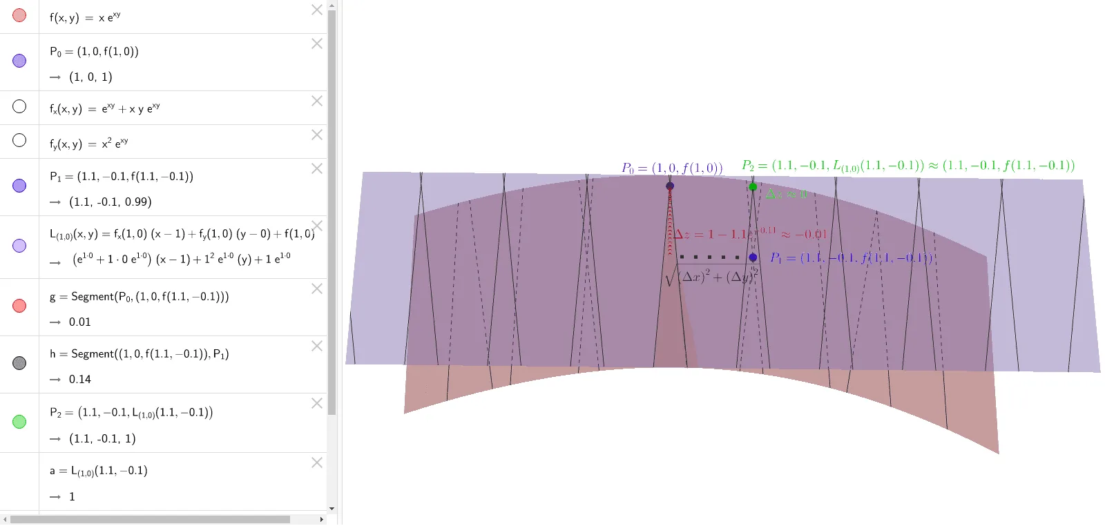
This example demonstrates how to plot tangent planes and linear approximations of a function in 3D space. Key math concepts include tangent plane equations, linear approximation, partial derivatives, and function graphing. GeoGebra commands used are Segment, objects like f (function), P0 (point), fx (partial derivative x), fy (partial derivative y), P1 (point), L(1,0) (line), g, h, P2 (point), a, b, P3 (point). Suitable for university calculus courses to help students understand the geometric meaning and applications of tangent planes and linear approximations.