Trapezoid Rule Demonstration

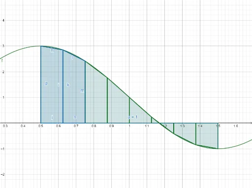
This example demonstrates the Trapezoid Rule for numerical integration, approximating the area under a function curve by dynamically constructing trapezoids. Key math concepts include numerical integration, trapezoidal approximation, function continuity, and geometric construction. GeoGebra commands and objects used, as per the construction summary, are Integral, Polygon, Sequence, with objects like f (function), a (lower limit), N (number of intervals), dx (step size), etc. Suitable for high school and above students learning numerical methods in calculus, or for teaching demonstrations of integral concepts.