Tangent Envelope and Derived Function Visualization

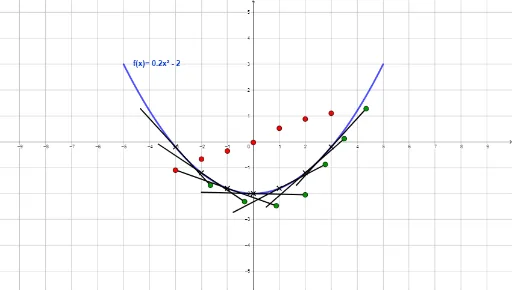
① This example dynamically displays the tangent lines at various points on a function curve, visually demonstrating the relationship between the tangent envelope and the derived function (derivative), where the slope of the tangent as a function of x forms the derivative graph. ② Core mathematical concepts include derivatives, tangent lines, envelopes, function graphs, and the geometric meaning of slope as instantaneous rate of change, central to calculus. ③ Construction highlights: using GeoGebra commands such as Circle, Point, Line, Slope, and Spline to construct the function curve, tangent points, tangent lines, and slope measurements; using Mirror and Segment for auxiliary symmetric or connecting elements; a Textfield allows input of the function expression; multiple points (A, B, C, etc.) and segments (l, m, n, etc.) are linked dynamically to produce a synchronized display of the tangent envelope and the derivative curve. ④ Suitable for high school to early college calculus instruction, helping students understand the definition of the derivative, tangent slope, and rate of change; also useful for classroom demonstrations or self-guided exploration of the geometric meaning of derivatives.